
Built-in Studies Reference Guide
The following document outlines the technical analysis theory for popular built-in studies.
Table of contents
- Accumulation/Distribution (A/D)
- Accumulative Swing Index (ASI)
- ADX/DMS
- Alligator
- Anchored VWAP
- Aroon
- Aroon Oscillator
- Average True Range (ATR)
- ATR Bands
- ATR Trailing Stop
- Awesome Oscillator (Awesome)
- Balance of Power
- Beta
- Bollinger Bands®
- Bollinger Bandwidth
- Bollinger %B
- Center of Gravity (COG)
- Chaikin Money Flow (CMF)
- Chaikin Volatility
- Chande Forecast Oscillator (CFO)
- Chande Momentum Oscillator (CMO)
- Choppiness Index
- Commodity Channel Index (CCI)
- Coppock Curve
- Correlation Coefficient
- Darvas Box
- Depth of Market
- Detrended Price Oscillator
- Disparity Index (DI)
- Donchian Channel
- Donchian Width
- Ease of Movement (EOM)
- Ehler Fisher Transform (EFT)
- Elder Force Index
- Elder Impulse System
- Elder Ray Index
- Fractal Chaos Bands
- Fractal Chaos Oscillator
- Gator Oscillator (GO)
- GoNoGo Trend
- Gopalakrishnan Range Index (GAPO)
- Guppy Multiple Moving Average
- High Low Bands
- High Minus Low
- Highest High Value (HHV)
- Historical Volatility
- Ichimoku Cloud (intro)
- Intraday Momentum Index
- Keltner Channel
- Klinger Volume Oscillator
- Linear Regression Forecast
- Linear Regression Intercept (LR-I)
- Linear Regression R2
- Linear Regression Slope
- Lowest Low Value (LLV)
- Market Facilitation Index (MFI)
- Mass Index (MI)
- Median Price
- Momentum
- Money Flow Index
- Moving Average
- Moving Average Convergence/Divergence (MACD)
- Moving Average Cross
- Moving Average Deviation
- Moving Average Envelope
- Negative Volume Index
- On Balance (Cumulative) Volume (OBV)
- Option Sentiment by Strike
- Parabolic SAR
- Performance Index (PI)
- Pivot Points
- Positive Volume Index (PVI)
- Pretty Good Oscillator
- Price Momentum Oscillator (PMO)
- Price Oscillator
- Price Rate of Change
- Price Relative (Relative Strength)
- Price Volume Trend (PVT)
- Prime Number Bands (PNB)
- Prime Number Oscillator
- Pring’s Know Sure Thing (KST)
- Pring’s Special K
- Projected Aggregate Volume (PAV)
- Projected Volume at Time (PVAT)
- Psychological Line (PL)
- QStick
- Rainbow Moving Average (RMA)
- Rainbow Oscillator (RO)
- Random Walk Index (RWI)
- Rapid Adaptive Variance Indicator (RAVI)
- Relative Strength
- Relative Strength Index (RSI)
- Relative Vigor Index (RVI)
- Relative Volatility
- Schaff Trend Cycle (STC)
- Shinohara Intensity Ratio (SIR)
- Standard Deviation
- STARC Bands
- Stochastics
- Stochastic Momentum (SMI)
- Supertrend
- Swing Index (SI)
- Time Series Forecast
- Trade Volume Index (TVI)
- Trend Intensity Index (TII)
- TRIX Oscillator
- True Range (TR)
- Twiggs Money Flow (TMF)
- Typical Price (TP)
- Ulcer Index
- Ultimate Oscillator
- Valuation Lines
- Vertical Horizontal Filter (VHF)
- Volatility Cone
- Volume Chart
- Volume Oscillator (VO)
- Volume Profile
- Volume Rate of Change
- Volume Underlay
- Volume Weighted Average Price (VWAP)
- Vortex Indicator (VI)
- Weighted Close (WC)
- Williams %R
- ZigZag
Accumulation/Distribution (A/D)
Indicator Type
Trend Analysis, Money Flow
Description
The Accumulation/Distribution (A/D) indicator calculates the strength of the market over time, based on the net change in price for each period compared to its prior period. When the net change is positive, the maximum difference between the close and the low or the close and the prior close is added to the A/D. Conversely, if the net change is negative the maximum difference between the close and the high or the prior close is subtracted from the A/D.
You can use the A/D to analyze money flow. In this case, the positive or negative direction is multiplied by the volume for the current period.
Note: The A/D uses all the data loaded into the chart. Typically this is 200 bars prior to the first bar shown. As the chart is compressed or panned it will load more data forcing the A/D to recalculate and will produce different values. That said, the pattern of the A/D will remain the same.
Math
- Input Parameter
- Use Volume
- todayAD:
- if Close(i)>Close(i-1) then
todayAD(i)=Close(i)-min(Low(i),Close(i-1))
- else if Close(i)<Close(i-1) then todayAD(i)=Close(i)-max(High(i),Close(i-1))
- else todayAD(i)=0
- If user selects “Use Volume”: todayAD(i)=todayAD(i)*Volume(i)
- if Close(i)>Close(i-1) then
todayAD(i)=Close(i)-min(Low(i),Close(i-1))
- R(i) = todayAD(i)+todayAD(i-1)+todayAD(i-2)+…+TodayAD(1)
Accumulative Swing Index (ASI)
Indicator Type
Trend Analysis
Description
The Accumulative Swing Index indicator (ASI) aggregates all the prior Swing Index (SI) values providing a longer term tool to support a swing trading strategy. The ASI is designed to help simplify market interpretation and leverage the sensitivity of the SI which helps detect potential changes in trend.
Note: The ASI uses all the data loaded into the chart. Typically this is 200 bars prior to the first bar shown. As the chart is compressed or panned it loads more data forcing the ASI to recalculate and will produce different values. That said, the pattern of the ASI will remain the same.
The Accumulative Swing Index was developed by Welles Wilder.
Related Study: Swing Index
Math
- T = Limit Move Value; if not supplied, 99999
- A(i) = abs(High(i)-Close(i-1))
- B(i)=abs(Low(i)-Close(i-1))
- C(i)=abs(High(i)-Low(i))
- D(i)=abs(Close(i-1)-Open(i-1))
- K(i)=max(A(i),B(i))
- M(i)=max(C(i),K(i))
- r(i)=M(i)+D(i)/4
- if M=A then r(i)=r(i)-B(i)/2
- else if M=B then r(i)=r(i)-A(i)/2
- S(i)=(50*((Close(i)-Close(i-1))+(Close(i)-Open(i))/2+(Close(i-1)-Open(i-1))/4)/r(i))*K(i)/T
- Swing Index: R(i)=S(i)
- Accumulative Swing Index: R(i)=R(i-1)+S(i)
ADX/DMS
Indicator Type
Trend Analysis, Momentum Oscillator
Description
ADX (Average Directional Index) or DMS (Directional Movement System) uses Directional Movement (DM) calculations to identify trends and gauge the strength of those trends. Directional Movement (DM) is defined as the largest part of the current period’s price range that lies outside the previous period’s price range. Each period will either be positive (PDM = larger range above previous range), negative (NDM = larger range below previous range), or zero if moves above and below the previous period’s range are equal or price stays within the previous day’s range (an inside bar).
A smoothed average of both positive and negative directional movement are calculated and then divided by the Average True Range (ATR) to derive the Plus Directional Indicator (+DI) and Minus Directional Indicator (-DI). Each period will have only one result, either plus, minus or zero. +DI increases and -DI decreases during rising trends and vice-versa in down trends. The DI Difference (DI) is the sum of +DI and -DI. Accordingly, the DI Histogram will oscillate around zero as the market trends.
The Average Directional Index (ADX) is a simple moving average of the absolute value of the DI. The ADX is a non-directional trend analysis tool. Low values indicate the market has consolidated and is ready to trend, whereas high values indicate a strong trend has been well established and may be nearing an end.
The ADX/DMS study displays the ADX line as well as the +DI and -DI. In addition, there is an option to display a histogram of the spread between +DI and -DI which serves as a momentum oscillator.
Formula
-
Directional Movement (DM) is defined as the largest part of the current period’s price range that lies outside the previous period’s price range.
- PDM = current high minus the previous high (called plus DM)
- MDM = current low minus the previous low (called minus DM)
- If PDM > MDM then MDM is set to zero
- If MDM > PDM then PDM is set to zero
- If current range lies within or is equal to the previous range then set both PDM and MDM to zero
-
Calculate the value of the Plus and Minus Directional Indicators:
- PDI(n) = PDM(n) * 100 ÷ ATR(n)
- MDI(n) = MDM(n) * 100 ÷ ARR(n)
- Where: n = Number of periods
- ATR = Average True Range
-
Calculate the absolute value of the Directional Movement Index (DMI):
- DMI = (PDI – MDI) ÷ (PDI + MDI)
-
Calculate the Average Directional Movement (DMIA a.k.a. ADX):
- DMIA(n) = SMA of DMI
Math
- Input Parameters
- Period (N)
- Smoothing Period (Sm)
- Display Settings
- Series (Show/Hide)
- Shading (Show/Hide)
- Histogram (Show/Hide)
- Sm=N unless user specified, this is ADX Smoothing period
- TR(i)=True Range (max(High(i),Close(i-1))-min(Low(i),Close(i-1)))
- pDM(i)=max(0,High(i)-High(i-1))
- nDM(i)=max(0,Low(i-1)-Low(i))
- if pDM(i)>nDM(i), then nDM(i)=0
- if(nDM(i)>pDM(i), then pDM(i)=0
- if(pDM(i)=nDM(i), then pDM(i)=0 and nDM(i)=0
- if i<=N:
- spDM(i)=spDM(i-1)+pDM(i)
- snDM(i)=snDM(i-1)+nDM(i)
- sTR(i)=sTR(i-1)+TR(i)
- else:
- spDM(i)=spDM(i-1)-spDM(i-1)/N+pDM(i)
- snDM(i)=snDM(i-1)-snDM(i-1)/N+nDM(i)
- sTR(i)=sTR(i-1)-sTR(i-1)/N+TR(i)
- if i>=N:
- pDI(i)=100*spDM(i)/sTR(i)
- nDI(i)=100*snDM(i)/sTR(i)
- DX(i)=100*abs(pDI(i)-nDI(i))/(pDI(i)+nDI(i))
- if i=Sm+N-1:
- R(Sm+N-1)=(DX(Sm+N-1)+DX(Sm+N-2)+DX(Sm+N-3)+…+DX(Sm))/Sm
- else:
- R(i)=(R(i-1)*(Sm-1)+DX(i))/Sm
- Histogram: pDI(x) – nDI(x)
Alligator
Indicator Type
Moving Averages/Bands
Description
The Alligator indicator uses three smoothed moving averages (SMMAs) named Jaw, Teeth, and Lips. Each one is offset forward (into the future) to indicate convergence/divergence relationships. The SMMAs are calculated on the Median Price. When the market is trending, the Alligator lines will diverge. When the three lines are close together, the Alligator indicates consolidation. The Gator oscillator is often used as a companion study to better understand the divergence/convergence between the three SMMAs.
The Alligator study can hide its Jaw, Teeth, and Lips lines, enabling users to show only the Fractal Arrows to emphasize trading signals.
The Alligator indicator was invented by Bill Williams.
Related Study: Gator Oscillator (GO)
Formula
Calculate three moving averages and offset them into the future.
- The Jaw line a 13-period SMMA, moved by 8 bars into the future;
- The Teeth line is an 8-period SMMA, moved by 5 bars into the future;
- The Lips line is a 5-period SMMA, moved by 3 bars into the future.
Math
- Input Parameters
- Jaw Period (Nj)
- Jaw Offset (Oj)
- Teeth Period (Nt)
- Teeth Offset (Ot)
- Lips Period (Nl)
- Lips Offset (Ol)
- Display Settings
- Lines (Show/Hide)
- Fractals (Show/Hide)
- Alligator Results:
- Rj(i)=SMMA(i-Oj,MP,Nj) //MP=Median Price
- Rt(i)=SMMA(i-Ot,MP,Nt)
- Rl(i)=SMMA(i-Ol,MP,Nl)
- Alligator Fractals:
- High(i)>max(High(i-1), High(i-2), High(i+1), High(i+2))
- Low(i)<min(Low(i-1), Low(i-2), Low(i+1), Low(i+2))
Anchored VWAP
Indicator Type
Volume, Moving Averages/Bands
Description
Anchored VWAP derives the volume-weighted average price (VWAP) starting from a specified date and time. Unlike VWAP, the Anchored VWAP can be applied to both intraday and historical price data. The mean of the high, low, and close price is the default price used to derive Anchored VWAP.
Related Study: Volume Weighted Average Price (VWAP)
Math
See VWAP
Aroon
Indicator Type
Trend Analysis
Description
The Aroon indicator measures the strength of a trend based on the recency of new Highs/Lows. Aroon plots two lines: the Aroon Up is based on recent highs and Aroon Down is based on recent lows. The values shown are in percentage terms and fluctuate between 0 and 100.
Related Study: Aroon Oscillator
Formula
- Parameters: Period (n)
- Aroon Up = 100 x (n – Days Since n-day High)/n
- Aroon Down = 100 x (n – Days Since n-day Low)/n
Math
- Input Parameters
- Period (N)
- For i = 0 to N-1 find Highest High’s index and Lowest Low’s index
- Xdh = index of HHV(i+1,N) includes current bar
- Xdl = index of LLV(i+1,N) includes current bar
- Rup(i) = 100*(1-(i-xdh)/N)
- Rdn(i) =100*(1-(i-xdl)/N)
Aroon Oscillator
Indicator Type
Momentum Oscillator
Description
The Aroon Oscillator measures the difference between Aroon Up and Aroon Down. The Aroon Oscillator is bounded between 100 and -100.
Related Study: Aroon
Formula
-
Parameters: Period (n)
-
Aroon Oscillator = Aroon Up – Aroon Down
Math
- Input Parameters
- Period (N)
- For i=0 to N-1 find Highest High’s index and Lowest Low’s index
- xdh=index of HHV(i+1,N) includes current bar
- xdl=index of LLV(i+1,N) includes current bar
- Rup(i)=100*(1-(i-xdh)/N)
- Rdn(i)=100*(1-(i-xdl)/N)
- Rosc(i)=Rup(i)-Rdn(i)
ATR Bands
Indicator Type
Moving Averages/Bands
Description
The ATR Bands indicator displays two lines forming an envelope around the Price series (X) based on recent volatility as measured by Average True Range (ATR). The Bands are calculated using a ±Shift multiple of the ATR and added/subtracted from X. When the price breaks out of the channel, it can be interpreted as a signal.
Related Study: Average True Range (ATR), ATR Trailing Stop, True Range (TR)
Note: This study can be applied to other studies by using the Field parameter.
Formula
- Parameters: Period (N); %Shift
- Top Band = Median Band + %Shift * ATR(N)
- Bottom Band = Median Band - %Shift * ATR(N)
Math
- Input Parameters
- Period (N)
- Field (X) //Any value displayed on the chart
- Shift (S)
- Display Settings
- Channel Fill (On/Off)
- Rm(i) (median band) = X(i)
- Rt(i) (top band) = Rm(i)+(S*ATR(i))
- Rb(i) (bottom band) = Rm(i)-(S*ATR(i))
ATR Trailing Stop
Indicator Type
Support/Resistance, Volatility
Description
ATR Trailing Stop highlights a reversal in trend by plotting a stop point based upon recent market volatility. Average True Range (ATR) is used to adjust the stop point based upon recent market volatility. The trailing stop will continue to increase in a rising market, and decrease in a down market. If the trend stalls or the market consolidates, the stop will stabilize at a level until the trend resumes or crosses through the stop level. ATR Trailing Stop flips to the invert when price corrects below/above the stop line.
Calculate the ATR and then apply the multiplier. For an up trend, subtract from previous close. For a down trend, add to the previous close.
Related Study: Average True Range (ATR), ATR Bands, True Range (TR)
Formula
(See Average True Range)
Math
- Input Parameters
- Period (N)
- Multiplier (M)
- HighLow (On/Off)
- Display Settings
- Plot Type
- base(i) = Close(i-1)
- offset(i) = ATR(i-1)*M (M is user supplied)
- if Close(i-1)>R(i-1) and Close(i-2)>R(i-1):
- if using High/Low, base(i)=High(i-1)
- R(i)=max(R(i-1),base(i)-offset(i))
- else if Close(i-1)<=R(i-1) and Close(i-2)<=R(i-1):
- if using High/Low, base(i)=Low(i-1)
- R(i)=min(R(i-1),base(i)+offset(i))
- else if Close(i-1)>R(i-1):
- if using High/Low, base(i)=High(i-1)
- R(i)=base(i)-offset(i)
- else if Close(i-1)<=R(i-1):
- if using High/Low, base(i)=Low(i-1)
- R(i)=base(i)+offset(i)
Average True Range (ATR)
Indicator Type
Volatility
Description
The Average True Range (ATR) is a simple moving average of the volatility of the market as measured by the True Range (TR).
Related Study: ATR Bands, ATR Trailing Stop, True Range (TR)
Formula
ATR = SMA( True Range, n-period )
Math
-
Input Parameters
- Period (N)
-
TR(i) = True Range
-
R(i) = (R(i-1)*(N-1)+TR(i))/N
Awesome Oscillator (Awesome)
Indicator Type
Momentum Oscillator
Description
The Awesome Oscillator measures the difference between a 5 period simple moving average (SMA) and a 34 period SMA based on the median price of each bar. The result is an unbounded oscillator. The Awesome is displayed as a histogram and each value is colored based on if the Awesome value is increasing or decreasing to provide visual clarity.
Related Study: Price Oscillator
Math
-
MP = (Highest Price + Lowest Price)/2
-
ma1(i) = SMA(i,MP,5)
-
ma2(i) = SMA(i,MP,34)
-
R(i) = ma1(i) - ma2(i)
-
Data is displayed as histogram:
-
if R(i) > R(i-1) use INCREASING BAR color
-
if R(i) < R(i-1) use DECREASING BAR color
-
Balance of Power
Indicator Type
Momentum Oscillator
Description
The Balance of Power is a moving average of the internal strength of each bar. The internal strength is measured by deriving a ratio of each bar's close-open relative to its high-low range. The highest/lowest value for any bar 1/-1, which occurs if the market opens on the low and closes on the high, and vice-versa in a down market. If the close equals the open the value for the bar is zero, indicating the power is balanced between the bulls and the bears.
Math
-
Input Parameters
-
Period (N)
-
Moving Average Type (xMA)
-
-
R(i) = xMA(i,(Close-Open)/(High-Low),N)
Beta
Indicator Type
Volatility, Comparison
Description
Beta measures the volatility of returns for one security against those of a benchmark security, usually a market index. It is often used as a measure of risk of a security relative to the market. A Beta greater than 1.0 will tend to move up or down faster than the benchmark security.
Math
-
Input Parameters
-
Period (N)
-
Comparison Symbol (Comp)
-
-
BaseChg(i) = Close(i) ÷ Close(i-1)
-
CompChg(i) = Comp(i) ÷ Comp(i-1)
-
MABase(i) = SMA(i,BaseChg,N)
-
MAComp(i) = SMA(i,CompChg,N)
-
COVARn(i) = (BaseChg(i)-MABase(i)) * (CompChg(i)-MAComp(i))
-
VARn(i) = (BaseChg(i)-MABase(i))^2
-
R(i) = SMA(i,COVARn,N)/SMA(i,VARn,N)
Bollinger Bands®
Indicator Type
Moving Averages/Bands, Volatility
Description
The Bollinger Bands indicator displays two lines forming an envelope around a moving average of price. The upper and lower bands are determined by a number of standard deviations above and below the moving average. The expansion and compression of the bands highlight changes in volatility. Breakouts of the bands typically represent trading opportunities.
Bollinger Bands were created by John Bolinger.
Related Study: Bollinger Bandwidth, Bollinger %B
Note: This study can be applied to other studies by using the Field parameter.
Formula
-
Parameters: Period (N); Standard Deviations (S)
-
Middle Band = N-period moving average
-
Upper Band = N-period moving average + (N-period standard deviation of price x multiple)
-
Lower Band = N-period moving average – (N-period standard deviation of price x multiple)
Math
-
Input Parameters
-
Period (N)
-
Field (X)
-
Standard Deviations (S)
-
Moving Average Type (xMA)
-
-
Display Settings
- Channel Fill (On/Off)
-
Rm(i) (moving average) = xMA(i,X,N)
-
ts(i)=total shift=(S*STDEV(i,X,N,xMA)
Standard Deviation =
-
Calculate the average (mean) price for N periods
-
Subtract each price over N periods from the average price over N periods
-
Square each difference
-
Sum these squares
-
Divide this sum by N
-
Standard deviation = the square root of that number
-
-
Rt(i) (top band) = Rm(i)+ts(i))
-
Rb(i) (bottom band) = Rm(i)-ts(i))
Bollinger Bandwidth
Indicator Type
Volatility
Description
The Bollinger Bandwidth measures the difference (spread) between the upper and lower Bollinger Bands. As the market trends and price dispersion increases the bands will widen, thereby providing a measure of volatility. When the Bollinger Bandwidth is low, due to a market consolidation, it is often considered a setup for a trend.
Bollinger Bands were created by John Bolinger.
Related Study: Bollinger Bands®, Bollinger %B
Note: This study can be applied to other studies by using the Field parameter.
Formula
Bandwidth = (Upper Band – Lower Band) ÷ Central Moving Average * 100
Math
-
Input Parameters
-
Period (N)
-
Field (X) //Any value displayed on the chart
-
Standard Deviations (S)
-
Moving Average Type (xMA)
-
-
Rm(i) (median band) = xMA(i,X,N)
-
ts(i)=total shift=(S*STDEV(i,X,N,xMA)
-
Rt(i) (top band) = Rm(i)+ts(i))
-
Rb(i) (bottom band) = Rm(i)-ts(i))
-
Rw(i)=100*(Rt(i)-Rb(i))/ Rm(i) // can be represented as 200*ts(i)/Rm(i)
Bollinger %B
Indicator Type
Momentum Oscillator
Description
Bollinger %B is a percentage measure of a security’s location between the Bollinger Bands. %B can be lower than 0 or higher than 100 if price moves outside the bands which would be considered a breakout signal. A value of 50 implies the price is equal to the middle moving average.
Bollinger Bands were created by John Bolinger.
Related Study: Bollinger Bands®, Bollinger Bandwidth
Note: This study can be applied to other studies by using the Field parameter.
Formula
%B = (Price – Lower Band) ÷ (Upper Band – Lower Band)
Math
-
Input Parameters
-
Period (N)
-
Field (X) //Any value displayed on the chart
-
Standard Deviations (S)
-
Moving Average Type (xMA)
-
-
Display Settings
-
Overbought Threshold
-
Oversold Threshold
-
-
Rm(i) (median band) = xMA(i,X,N)
-
ts(i) (total shift) = (S*STDEV(i,X,N,xMA)
-
Rt(i) (top band) = Rm(i)+ts(i))
-
Rb(i) (bottom band) = Rm(i)-ts(i))
-
Rpb(i) = 50*(2*(Close(i)-Rm(i))/(Rt(i)-Rb(i))+1) // can be represented as ((Close(i)-Rm(i))/ts(i)+1)
Center of Gravity (COG)
Indicator Type
Momentum Oscillator
Description
The Center of Gravity (COG) is a leading oscillator created by John Ehlers in 2002. It is used to identify support and resistance. It is constructed using a weighted moving average, which according to its creator, was analogous to the weighted coordinates of an object’s mass distribution. It is accompanied by a Signal line.
Claiming to have zero lag, COG allows for clear indication of reversals due to the smoothing effect of the indicator. When the COG line crosses above the Signal line, it is an indication of an upturn. When the COG line crosses below the signal line, it is an indication of a market downturn.
Math
- Input Parameters
- Period (N)
- Field (X) //Any value displayed on the chart
- num(i) = 1*X(i)+2*X(i-1)+3*X(i-2)+…+N*X(i-N+1)
- den(i) = X(i)+X(i-1)+X(i-2)+…+X(i-N+1)
- R(i) = -num(i)/den(i)
Chaikin Money Flow (CMF)
Indicator Type
Money Flow
Description
The Chaikin Money Flow (CMF) indicator is a moving sum of volume which is weighted by where price closes within its range. The indicator oscillates around 0, with positive amounts indicating a bullish trend, and negative amounts indicating a bearish trend.
The weight is called a “multiplier”, which ranges from -1 for a close at the low to +1 for a close at the high. A multiplier of -1 implies all the volume is negative, and is subtracted from the moving sum. In contrast, if the multiplier equals +1, all the volume for the period is added to the moving sum.
The Chaikin Money Flow was developed by Marc Chaikin.
Related Study: On Balance (Cumulative) Volume (OBV), Twiggs Money Flow (TMF)
Formula
Money Flow Multiplier = ((Close–Low)–(High–Close)) / (High – Low)
Money Flow Volume = (Money Flow Multiplier) x Volume
CMF = (N-Period Sum of Money Flow Volume)/(N-Period Sum of Volume)
Math
- Input Parameters
- Period (N)
- MFV(i) = Volume(i)*(2*Close(i)-High(i)-Low(i))/(High(i)-Low(i))
- sMFV(i) = MFV(i)+MFV(i-1)+MFV(i-2)+…+MFV(i-N+1)
- sVol(i) = Volume(i)+Volume(i-1)+Volume(i-2)+…+Volume(i-N+1)
- R(i) = sMFV(i)/sVol(i)
Chaikin Volatility
Indicator Type
- Volatility
Description
Chaikin Volatility measures the rate of change, in percentage terms, of a moving average of the high-low range. Higher values indicate the volatility (as measured by range) has been increasing relative to itself. The values are unbounded.
The Chaikin Volatility was developed by Marc Chaikin.
Math
- Input Parameters
- Period (N)
- Rate of Change (ROC)
- Moving Average Type (xMA)
- ma(i) = xMA(i,High-Low,N)
- R(i) = 100*((ma(i)/ma(i-ROC))-1)
Chande Forecast Oscillator (CFO)
Indicator Type
Momentum Oscillator
Description
The Chande Forecast Oscillator (CFO) measures the spread, in percentage terms, between the market price and a Time Series Moving Average (TSMA) which is a n-period moving linear regression using the “least squares fit” method. The oscillator is above zero when the price is above the CFO and less than zero if it is below. The oscillator is quite responsive to changes in trend as the TSMA follows price quite closely.
The Chande Forecast Oscillator was introduced by Tushar Chande.
Related Study: Moving Average Deviation
Note: This study can be applied to other studies by using the Field parameter.
Math
- Input Parameters
- Period (N)
- Field (X) //Any value displayed on the chart
- T(i) = TSMA(i,X,N) //Time Series (TSMA)
- R(i) = 100*(1-T(i)/X(i))
Chande Momentum Oscillator (CMO)
Indicator Type
Momentum Oscillator
Description
The Chande Momentum Oscillator (CMO) compares, in percentage terms, the sum of all recent one-period price changes divided by the sum of the absolute values of the one-period price changes over the same time period. The range of the CMO is bounded between -100 and +100.
The Chande Momentum Oscillator was introduced by Tushar Chande and Stanley Kroll.
Math
- Input Parameters
- Period (N)
- Display Settings
- Show Zones (Show/Hide)
- OverBought
- OverSold
- mom(i) = Close(i)-Close(i-1)
- Sm(i) = mom(i)+mom(i-1)+mom(i-2)+…+mom(i-N+1)
- AbsSm = abs(mom(i))+abs(mom(i-1))+abs(mom(i-2))+…+abs(mom(i-N+1))
- R(i) = 100*Sm(i)/absSm(i)
Choppiness Index
Indicator Type
Trend Analysis, Volatility
Description
The Choppiness Index (CI) is a non-directional trend analysis indicator which rises during a consolidation and falls as the market trends. The CI is a bounded range between 0 - 100. The higher the value, the less the market is trending.
The Choppiness Index was created by Australian commodities trader E.W. Driess.
Math
- Input Parameters
- Period (N)
- Display Settings
- Show Zones (Show/Hide)
- OverBought
- OverSold
- sTR(i) = TR(i)+TR(i-1)+TR(i-2)+…+TR(i-N+1)
- hh = HHV(i+1,N) //Highest High starting at current bar
- ll = LLV(i+1,N) //Lowest Low starting at current bar
- R(i) = 100*ln(sTR(i)/(hh-ll))/ln(N)
Commodity Channel Index (CCI)
Indicator Type
Momentum Oscillator
Description
The Commodity Channel Index (CCI) study measures market momentum by deriving a price oscillator and normalizing it by the deviation of price from its average. Specifically, it uses the average of the high, low and close for the period (HLC3, also referred to as “typical price”) and subtracts the “n” period moving average of HLC3, this quantity is then divided by the mean deviation of price from the simple moving average (SMA). By measuring price relative to its SMA, the CCI effectively captures the acceleration and deceleration of a market trend.
CCI is an unbounded oscillator. A factor of 0.015 is used to center the series so that +100 and -100 (default threshold values) may be used to identify Overbought and Oversold conditions. When CCI equals 0 it indicates that price is equal to the SMA. The Commodity Channel Index was developed by Donald Lambert.
Formula
Typical Price = (high + low + close) ÷ 3
CCI = Typical Price (TP) – (n-period SMA of TP) ÷ (0.015 * Mean Deviation)
Mean Deviation = ∑ (absolute value of difference of TP and its N-pd SMA) ÷ N
Math
- Input Parameters
- Period (N)
- TP(i) = Typical Price
- a(i) = SMA(i,TP,N)
- md(i) = abs(TP(i)-a(i))+abs(TP(i-1)-a(i)) + abs(TP(i-2)-a(i))+…+abs(TP(i-N+1)-a(i))
- R(i) = N*(TP(i)-SMA(i,TP,N))/(.015*md(i))
Coppock Curve
Indicator Type
Momentum Oscillator
Description
The Coppock Curve is calculated by first summing two rate of change measures, one with a long period and second with a short period. The Coppock Curve is a weighted moving average of this sum.
The Coppock Curve was created by Edwin Coppock.
Note: This study can be applied to other studies by using the Field parameter.
Formula
-
Parameters: Short RoC Period, Long RoC Period, MA Period
-
RoCSum = 100 * ( (Short RoC) + (Long RoC) - 2 )
-
Coppock = WMA( RoCSum,N )
Math
- Input Parameters
- Period (N)
- Field (X) // Any value displayed on the chart
- Short RoC (N1)
- Long RoC (N2)
- s(i) = 100*((X(i)/X(i-N1)) + (X(i)/X(i-N2))-2)
- R(i)= WMA(i,s,N)
Correlation Coefficient
Indicator Type
Statistical, Relative performance measure, Comparison
Description
The Correlation Coefficient is a statistical measure used to calculate the strength and direction of the linear relationship (or the statistical relationship) between two data sets. For charting, it is between two traded instruments and the result is recalculated for each period in the same way a moving average “moves” through time using fresh data.
The value ranges between -1 to +1. The positive and negative correlation coefficient represents the direct (positive) and inverse (negative) linear correlation or statistical relationship between the data sets. That is, a positive correlation indicates two instruments have traded in the same direction, whereas a negative correlation implies they have traded in opposite directions. If the correlation is close to zero or equal to zero then the data sets are considered uncorrelated.
Formula
In the formula, the symbols μx and μy represent the mean of the two data sets X and Y respectively. The σx and σy represents the sample standard deviation of the two data sets X and Y respectively.
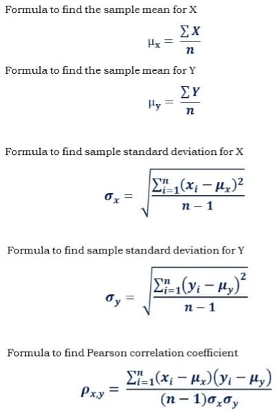
Step by Step Calculation:
- Find the sample mean μx for data set X.
- Find the sample mean μy for data set Y.
- Estimate the standard deviation σx for sample data set X.
- Estimate the sample deviation σy for data set Y.
- Find the covariance (cov(x, y)) for the data sets X and Y.
- Apply the values in the formula for correlation coefficient to get the result.
Math
- Input Parameters
- Comp=Close of the comparison symbol
- Period (N)
- sB(i)=Close(i)+Close(i-1)+Close(i-2)+…+Close(i-N+1)
- sC(i)=Comp(i)+Comp(i-1)+Comp(i-2)+…+Comp(i-N+1)
- sB2(i)=(Close(i)^2)+(Close(i-1)^2)+Close(i-2)^2)+…+Close(i-N+1)^2)
- sC2(i)=(Comp(i)^2)+(Comp(i-1)^2)+Comp(i-2)^2)+…+Comp(i-N+1)^2)
- sBC(i)=Close(i)*Comp(i)+Close(i-1)*Comp(i-1)+Close(i-2)*Comp(i-2)+…+Close(i-N+1)*Comp(i-N+1)
- vb=sB2(i)/N-((sB(i)/N)^2)
- vc=sC2(i)/N-((sC(i)/N)^2)
- cv=sBC(i)/N-sB(i)*sC(i)/(N^2)
- R(i)=cv/((vb*vc)^.5)
Darvas Box
Indicator Type
Support/Resistance
Description
The Darvas Box is a support/resistance indicator and a trading methodology rolled into one. It is an overlay study meant to indicate stocks that are trading at new highs by highlighting recent highs and lows to indicate entry points and placement of stop-losses.
The rules of drawing the Darvas Box are:
- Boxes are drawn around bars where an “all time high” was reached followed by 3 successive higher lows, and the high of the first bar was not broken by a higher high
- The box continues until either the original high is broken out, or the lowest of the 2 successive lows is broken below
- User can configure if high/low or close breaks the box
- User can configure if “Ghost boxes” are shown
- These will form on an upwards breakout of a Darvas
- The low of the Ghost box will be the same value as the high of the Darvas which was broken
- The height of the Ghost box will be the same as the Darvas box
- The width of the Ghost box will be either:
- The width of the Darvas box
- Until the Ghost box is broken below
- Until the Ghost box is broken above, in which case
- Another Ghost box forms with the lower left corner at the upper right corner of the preceding Ghost box
- User can define if arrow is drawn pointing to a volume spike and at what percentage that will be
- User can configure period defining all time high
- User can define a price minimum below which boxes will not form
- User can define whether “Stop Levels” are drawn and how far below the box low. Stop levels cannot be lowered, only raised (or broken).
While the indicator will run on any bar interval it is best used on higher intervals (i.e., weekly/monthly) with securities in a strong trend.
The logic behind the construction of the Darvas Box is somewhat complex but the usage is fairly straightforward. Once you have a closed box (a blue box assuming the default settings) you wait for a close (or a high) above the box on higher volume for a bullish signal or a close (or a low) below the box on higher volume for a bearish signal. The stop would generally be set just past the other side of the box. New boxes which form while you are in a trade provide an opportunity to build on a position upon a new breakout as well as updating a trailing stop level based on the most recent box. When used strictly as an indicator, the Darvas Box is an excellent mechanism to identify trading ranges on all bar intervals.
Depth of Market
Indicator Type
Volume
Detrended Price Oscillator
Indicator Type
Trend Analysis
Description
The Detrended Price Oscillator (DPO) seeks to remove trend information from the data. It does this by taking a moving average and shifting it to the left. It then subtracts the average from the time period from the close of that time period to arrive at the result.
The DPO will not be displayed on the most recent period as the moving average is shifted to the left. The resulting DPO plot will emphasize the movement of the security above and below the moving average while filtering out the general trends. The DPO is often used to help find cycles in the market by identifying peaks and troughs.
Note: This study can be applied to other studies by using the Field parameter.
Formula
The Moving Average type defaults to Simple, and the moving average period defaults to 14, computed on the Close.
N is the period, and X is the data field.
-
MA = xMA(i, X, N)
-
MAShifted = MA(i+int(N/2+1)) // where “int” is the whole number portion of the formula. For example, int(16.5)=16.
-
DPOi = Xi - MAShifted
Math
-
Input Parameters
-
Period (N)
-
Field (X) // Any value displayed on the chart
-
Moving Average Type (xMA)
-
-
R(i) = X(i)-xMA(i+int(N/2+1),X,N)
-
Moving average is shifted to the left
Disparity Index (DI)
Indicator Type
Momentum Oscillator
Description
The Disparity Index (DI) measures the distance of price from a moving average in percentage terms. The DI is an unbounded oscillator that uses percentage based calculation to normalize the spread across time and price.
Related Study: Moving Average Deviation
Note: This study can be applied to other studies by using the Field parameter.
Formula
- DI = Price ÷ Moving Average - 1
Math
-
Input Parameters
-
Period (N)
-
Field (X) // Any value displayed on the chart
-
Moving Average Type (xMA)
-
-
ma(i) = xMA(i,X,N)
-
R(i) = 100*(X(i)/ma(i)-1)
Donchian Channel
Indicator Type
Moving Averages/Bands
Description
The Donchian Channel displays a median line and bands that form an envelope around price. The Donchian High is the Highest High and the Donchian Low is the Lowest Low of the prior n periods starting with the previous bar. The median line is the average of the Donchian High and Donchian Low bands for each period.
The Donchian Channel was developed by Richard Donchian.
Related Study: Donchian Width, Highest High Value (HHV), Lowest Low Value (LLV)
Math
-
Input Parameters
-
High Period (Nh)
-
Low Period (Nl)
-
-
Display Setting
- Channel Fill (Show/Hide)
-
hh = HHV(i,Nh) // Highest High Value starts at previous bar
-
ll = LLV(i,Nl) // Lowest Low Value starts at previous bar
-
Rt(i) = hh
-
Rb(i) = ll
-
Rm(i) = (hh+ll)/2
Donchian Width
Indicator Type
- Volatility
Description
The Donchian Width indicator measures the spread between the Donchian High and Donchian Low bands. This serves as a simple measure of volatility as it captures the range expansion/compression of the market.
The Donchian Channel was developed by Richard Donchian.
Related Study: Donchian Bands, Highest High Value (HHV), Lowest Low Value (LLV)
Math
-
Input Parameters
-
High Period (Nh)
-
Low Period (Nl)
-
-
hh = HHV(i,Nh) // Highest High Value starts at previous bar
-
ll = LLV(i,Nl) // Lowest Low Value starts at previous bar
-
Rw(i) = hh-ll
Ease of Movement (EOM)
Indicator Type
- Money Flow, Trend Analysis, Momentum Oscillator
Description
The Ease of Movement (EOM) indicator is designed to measure volume’s impact on price. EOM first divides the volume by the period’s high-low Range, essentially distributing the volume equally across the high-low range. This value is then used as the denominator to measure the impact on the price change. A large change in price implies the volume was able to move the market.
EOM is an unbounded oscillator. A rising EOM indicates the market is easily moving upward, and the converse is true on the downside.
The Ease of Movement indicator was developed by Richard W. Arms, Jr.
Formula
EOM = Moving Average ( 1 bar Price Change ÷ ( Volume ÷ H-L Range ) )
Math
-
Input Parameters
-
Period (N)
-
Moving average Type (xMA)
-
-
ac(i) = (High(i)-Low(i))/2
-
ap(i) = (High(i-1)-Low(i-1))/2
-
dm(i) = ac(i)-ap(i) //Change in Midpoint
-
br(i) = (Volume(i)/100000000)/(High(i)-Low(i))
-
e(i) = dm(i)/br(i)
-
R(i) = xMA(i,e,N)
Ehler Fisher Transform (EFT)
Indicator Type
- Momentum Oscillator
Description
The Ehler Fisher Transform (EFT) is designed to convert prices into a Gaussian normal distribution based on the recent n-period trading range. The EFT is an unbounded oscillator with a trailing Trigger line that is the EFT with a lag of 1 period. The EFT is designed to reduce volatility of the indicator, but still provide timely signals of change in trend.
The Fisher Transform is a technical indicator created by John F. Ehlers
Math
-
Input Parameters
- Period (N)
-
hh=HHV(i+1,N) //Highest High starting at current bar
-
ll=LLV(i+1,N) //Lowest Low starting at current bar
-
n:
-
n(0)=0
-
n(i)=0.33*2*((((High(i)+Low(i))/2)-ll)/(hh-ll)-0.5)+0.67*n(i-1)
-
n(i)=min(max(n,-.9999),.9999)
-
-
R(i) = .5*ln((1+n)/(1-n))+.5*R(i-1)
-
Trigger(i) = R(i-1)
Elder Force Index
Indicator Type
- Money Flow, Momentum Oscillator
Description
The Elder Force Index (EFI) is a money flow based oscillator that multiplies the period’s volume times the price change thereby showing the strength of the price movement. EFI is an unbounded oscillator. A rising EFI indicates volume is driving prices higher, and a declining EFI indicates volume is pushing the market lower.
The Elder Force Index was developed by Alexander Elder.
Formula
-
Parameters: Period
-
EFI = EMA (Volume * 1 period Price Change, N-Period )
Math
-
Input Parameters
- Period (N)
-
EF1(i) = Volume(i)*(Close(i)-Close(i-1))
-
R(i) = EMA(i,EF1,N)
Elder Impulse System
Indicator Type
Trend Analysis
Description
The Elder Impulse System (EIS) combines net changes in an exponential moving average (EMA) of price with net changes in the MACD histogram to produce bullish and bearish signals applied to the chart using paintbars. The result is a colored bar chart where the colors represent bullish, bearish or neutral signals. Bullish (green) signals appear when the values of both the EMA and the MACD Histogram increase from the prior period. Conversely, if both decrease then it is a bearish (red) signal. If they move in opposite directions then it is a neutral signal (blue).
The Elder Impulse System was developed by Alexander Elder.
Formula
-
The study parameters in the EIS are fixed as follows:
-
EMA had a period of 13, computed on the Close.
-
The MACD has a fast period of 12, a slow period of 26, and a signal period of 9.
-
Math
-
ma(i) = EMA(i,Close,13)
-
cdh(i) = MACD(i,12,26,9) Histogram // This is the MACD-MACDSignal
-
if ma(i)>ma(i-1) and cdh(i)>cdh(i-1) then bullish
-
if ma(i)<ma(i-1) and cdh(i)<cdh(i-1) then bearish
-
display colored bar chart, bullish color if bullish, bearish color if bearish, otherwise neutral color
Elder Ray Index
Indicator Type
- Momentum Oscillator
Description
The Elder Ray Index is an unbounded oscillator that displays two superimposed histograms measuring the distance of the high/low from the exponential moving average.
The Elder Ray Index was developed by Alexander Elder.
Formula
-
Parameters: Period
-
Bull Power = High - EMA (Close, N-Period)
-
Bear Power = Low - EMA (Close, N-Period)
Math
-
Input Parameters
- Period (N)
-
Histogram1(i) = High(i) - EMA(i,Close,N)
-
Histogram2(i) = Low(i) - EMA(i,Close,N)
Fractal Chaos Bands
Indicator Type
- Moving Average/Bands, Trend Analysis
Description
The Fractal Chaos Bands are designed to identify breakouts and trend persistence based on the market making new Highs/Lows. An upside breakout is identified when the current high is the Highest High when compared to the prior two highs, in which case the Upper Band holds its last value and moves sideways. If the market is not trending, either up or down, then the Upper Band will display the high from two bars ago. The reverse is done for the Lower Band.
Related Study: Fractal Chaos Oscillator
Math
-
if High(i)<High(i-2) and High(i-1)<High(i-2) and going back, found 2 more Highs<High(i-2) before finding any>High(i-2) then
- Rh(i)=High(i-2)
-
if Low(i)>Low(i-2) and Low(i-1)>Low(i-2) and going back, found 2 more Lows>Low(i-2) before finding any<Low(i-2) then
- Rl(i)=Low(i-2)
Fractal Chaos Oscillator
Indicator Type
Momentum Oscillator
Description
The Fractal Chaos Oscillator has three states -1, 0, +1. A value of 0 indicates the market is consolidating. A value of +1 indicates a change in the upper range of the market, as best seen using the Upper Fractal Chaos Band. A value of -1 indicates a change in the lower range of the market, as best seen using the Lower Fractal Chaos Band.
The Fractal Chaos Oscillator was developed by E. W. Dreiss.
Related Study: Fractal Chaos Bands
Math
-
if High(i)<High(i-2) and High(i-1)<High(i-2) and going back, found 2 more Highs<High(i-2) before finding any>High(i-2) then
-
Rh(i)=High(i-2)
-
Rosc(i)=1
-
-
if Low(i)>Low(i-2) and Low(i-1)>Low(i-2) and going back, found 2 more Lows>Low(i-2) before finding any<Low(i-2) then
-
Rl(i)=Low(i-2)
-
Rosc(i)=-1
-
-
if neither of the two conditions above,
- Rosc(i)=0
Gator Oscillator (GO)
Indicator Type
Oscillator, Trend Analysis
Description
The Gator Oscillator (GO) is derived from the Alligator indicator. It plots two histograms in opposite directions that highlight the divergence/convergence between the three SMMAs used in the Alligator: Jaws, Teeth, and Lips. The positive histogram is the absolute value of the (Jaw - Teeth). The negative histogram is the absolute value of the (Teeth - Lips) multiplied by -1.
Green histogram bars indicate the averages are diverging, highlighting acceleration of the trend. Red bars indicate convergence of the averages showing the trend is losing strength. Compression of the histograms helps determine when a market is consolidating.
Although the GO can be used separately, it is most often combined with the Alligator as they complement each other in giving a more complete overview of current market conditions. The GO shows the absolute degree of convergence/divergence of the three moving averages plotted by Alligator study.
Related Study: Alligator
Formula
Calculate three moving averages and offsets them into the future.
- The Jaw line a 13-period Smoothed Moving Average (SMMA), moved into the future by 8 bars;
- The Teeth line is an 8-period Smoothed Moving Average (SMMA), moved by 5 bars into the future;
- The Lips line is a 5-period Smoothed Moving Average, moved by 3 bars into the future.
- Gator Hist_1 = ABS( SMMA(median price,Jaws) - SMMA(median price, Teeth) )
- Gator Hist_2 = -1*ABS( SMMA(median price,Teeth) - SMMA(median price, Lips) )
Math
- Input Parameters
- Jaw Period (Nj)
- Jaw Offset (Oj)
- Teeth Period (Nt)
- Teeth Offset (Ot)
- Lips Period (Nl)
- Lips Offset (Ol)
- Alligator Results:
- Rj(i) = SMMA(i-Oj,MP,Nj) //MP=Median Price
- Rt(i) = SMMA(i-Ot,MP,Nt)
- Rl(i) = SMMA(i-Ol,MP,Nl)
- Gator Results (Histogram):
- Rjt(i) = abs(Rj(i)-Rt(i)) //Jaw-Teeth
- Rtl(i) = -abs(Rt(i)-Rl(i)) //Teeth-Lips
- if Rjt(i)>Rjt(i-1) use INCREASING BAR color
- if Rjt(i)<Rjt(i-1) use DECREASING BAR color
- if Rtl(i)>Rtl(i-1) use DECREASING BAR color
- if Rtl(i)<Rtl(i-1) use INCREASING BAR color
GoNoGo Trend
Indicator Type
- Trend Analysis
Description
The GoNoGo Trend study colors the price action of any security according to the strength of its trend, making it simple to identify and interpret the current trend:
-
Bright Blue price bars indicate the strongest bullish environment.
-
Aqua bars are slightly less bullish; they often occur at the start of a new trend, or as a strong bullish trend begins to weaken.
-
Amber bars represent uncertainty, often appearing in the transition from bull trend to bear trend and vice versa.
-
Pink bars indicate a lower intensity bearish environment
-
Dark Purple bars are shown when the bearish trend intensifies.
The “Go” and “NoGo” labels on the chart mark transitions to bull or bear trends, respectively.
Math
- Proprietary to GoNoGo Charts
Gopalakrishnan Range Index (GAPO)
Indicator Type
Volatility
Description
The Gopalakrishnan Range Index (GAPO) measures the volatility of the market by measuring the natural log of the spread between the Highest High and Lowest Low over a given period which is then normalized by the natural log. When the GAPO is increasing the market is making new highs or lows relative to the lookback period.
Formula
-
Parameter: Period (N)
-
GAPO = Natural Log(Highest High - Lowest Low) ÷ Natural Log(N)
Math
-
Input Parameters
- Period
-
hh = HHV(i,N) – Highest High starting at previous bar
-
ll = LLV(i,N) – Lowest Low starting at previous bar
-
R(i) = ln(hh-ll)/ln(N) - ln is the natural log
Guppy Multiple Moving Average
Indicator Type
Moving Averages/Bands
Description
The Guppy Multiple Moving Average (GMMA) combines a group of six short-term exponential moving averages (EMA) and a group of six long-term EMAs. The multiple moving averages provide a “weight of the evidence” approach to identify changing trends, breakouts, and trading opportunities in the price of an asset.
The Guppy Multiple Moving Average was introduced by Daryl Guppy.
Formula
-
Short Term (Red Averages)
-
EMA(3)
-
EMA(5)
-
EMA(8)
-
EMA(10)
-
EMA(12)
-
EMA(15)
-
-
Long Term (Blue Averages)
-
EMA(30)
-
EMA(35)
-
EMA(40)
-
EMA(45)
-
EMA(50)
-
EMA(60)
-
High Low Bands
Indicator Type
Moving Averages/Bands, Statistical
Description
The High Low Bands are drawn a percentage or number of points above and below a triangular moving average of the selected field.
Related Study: Triangular Moving Average, Moving Average Envelope
Math
-
Input Parameters
-
Period
-
Field
-
Shift Percentage
-
-
Creates a plot of the TMA plus 2 bands ±S percentage off the Close from the TMA
High Minus Low
Indicator Type
Volatility
Description
High Minus Low measures the trading range of the bar.
Related Study: True Range (TR)
Math
- R(i) = High(i)-Low(i)
Highest High Value (HHV)
Indicator Type
Statistical, Band
Description
Identifies the highest price over a defined range, excluding the current bar in order to highlight if the current price is exceeding the recent Highest High.
Related Study: Lowest Low Value (LLV)
Math
-
Input Parameters
- Period
-
Does not include current bar
-
R(i)=max(X(i-1),X(i-2),X(i-3),…,X(i-N)) //start at previous bar
Historical Volatility
Indicator Type
Volatility, Statistical
Description
Historical Volatility measures the standard deviation of the underlying percent returns over n-periods. The result is annualized.
Math
-
Input Parameters
-
Period (N)
-
Field (X) //Any value displayed on the chart
-
Days Per Year: Select 365 or 252 for Market Days in year for daily charts. For monthly charts there are 12 periods. For weekly charts 52 periods.
-
Standard Deviations (M)
-
-
AF = 100*(Number Periods in Year ^ .5)*M //Annualization Factor
-
L(i) = ln(X(i)/X(i-1))
-
avgL(i) = (L(i)+L(i-1)+L(i-2)+…+L(i-N+1))/N
-
d2(i) = ((L(i)-avgL(i))^2)+((L(i-1)-avgL(i))^2)+((L(i-2)-avgL(i))^2)+…+((L(i-N+1)-avgL(i))^2)
-
R(i) = ((d2(i)/N)^.5)*AF
Ichimoku Cloud
Indicator Type
Trend analysis, Support/Resistance
Description
The Ichimoku Cloud study is designed to indicate support/resistance, momentum, and trend direction. It plots five lines and computes various “clouds” based on the interactions between these lines. Ichimoku translates to “one look,” implying that the indicator can signal support and resistance at a glance.
There are five components:
- Tenkan Sen (Conversion Line) – Calculated as the sum of the Highest High over the past nine periods and the Lowest Low divided by two.
- The Kijun Sen (Base Line) – Calculated as the sum of the Highest High over the past 22 periods and the Lowest Low divided by two.
- Senkou Span A (leading) – The sum of the Tenkan Sen and the Kijun Sen divided by two. The calculation is then plotted 26 time periods ahead of the current price action.
- Senkou Span B (leading) – The sum of the Highest High and the Lowest Low over the past 52 periods divided by two. It is also plotted 26 periods ahead.
- Chikou (lagging) – The same and Senkou Span B leading but plotted 26 periods in the past.
Math
- 5 lines are drawn
- Conversion Line:
- Ncl=Conversion Line Periods
- Rcl(i)=(HHV(i+1,Ncl)+LLV(i+1,Ncl))/2 – include current period
- Base Line:
- Nbl=Base Line Periods
- Rbl(i)=(HHV(i+1,Nbl)+LLV(i+1,Nbl))/2 – include current period
- Lagging Span:
- Nlg=Lagging Span Periods
- Rlg(i)=Close(i-Nlg)
- Leading Spans:
- Nld=Leading Span Periods
- Rlda(i+Nld)=(Rcl(i)+Rbl(i))/2
- Rldb(i+Nld)=(HHV(i+1,Nld)+LLV(i+1,Nld))/2 – include current period
- “Clouds” are drawn between the Leading Spans as follows:
- Red cloud if Rldb(i)>Rlda(i)
- Green cloud if Rlda(i)>Rldb(i)
Intraday Momentum Index
Indicator Type
Momentum Oscillator
Description
The Intraday Momentum Index (IMI) measures trend strength by using a ratio of the moving sum of the close-open (candle body) over the past “n” periods and relative to the moving sum of the net decreases. The result is a bounded oscillator that is indexed between 0 and 100 and is displayed with Overbought (OB) and Oversold (OS) levels.
The methodology to calculate IMI is quite similar to the Relative Strength Indicator (RSI) and can be interpreted in a similar manner. The central difference between the two is IMI measures market strength/weakness using the range of close-open (hence, the use of ‘Intraday’ in the name) whereas RSI measures the one-period net change. An advantage of IMI is it tends to trend more smoothly and produces OB/OB levels more frequently.
Related Study: Relative Strength Index (RSI)
Math
-
Input Parameters
- Period (N)
-
Display Settings
-
Show Zones (On/Off)
-
OverBought
-
OverSold
-
-
d(i) = Close(i)-Open(i) //Candle body
-
p(i): max(0,d(i))
-
n(i): min(0,d(i))
-
totP(i) = totP(i-1)+totP(i-2)+totP(i-3)+…+totP(i-N+1)+p(i) //Sum of gains
-
totL(i) = totL(i-1)+totL(i-2)+totL(i-3)+…+totL(i-N+1)-n(i) //Sum of losses
-
R(i) = 100*(totP(i)/(totP(i)+totL(i))) //percent of point up vs losses
Keltner Channel
Indicator Type
Moving Averages/Bands
Description
The Keltner Channel indicator displays two lines forming an envelope around a moving average of price. The upper and lower channel lines are determined by adding/subtracting a multiple of the Average True Range above and below the moving average of price. The Keltner Channel highlights the expansion and compression of volatility.
Formula
-
Center Line: 50-day EMA
-
Upper Channel Line: 50-day EMA + (5 x ATR (10-period))
-
Lower Channel Line: 50-day EMA – (5 x ATR (10-period))
Math
- Input Parameters
- Period (N)
- Shift (%S)
- Moving Average Type (xMA)
- Display Settings
- Channel Fill (On/Off)
- Rm(i) = xMA(i,Close,N) //center line
- Rt(i) = Rm(i)+(%S*ATR(i)) //top channel
- Rb(i) = Rm(i)-(%S*ATR(i)) //bottom channel
Klinger Volume Oscillator
Indicator Type
Money Flow
Description
The Klinger Volume Oscillator (KVO) is designed to identify short term fluctuations in money flowing in or out of a security. Each period’s volume is assigned a positive or negative value based on the one period change in Typical Price (the mean of the high, low, and close). The KVO is the spread between a long and a short exponential moving average (EMA) of the directional volume series.
The Signal Line is simply an EMA of the KVO line. The KVO Histogram measures the spread between the KVO and the Signal line. The KVO Histogram is colored green when the values are increasing and red when they are decreasing (green and red are default colors).
KVO is useful in helping evaluate if volume is supporting the trend.
The KVO was developed by Stephen Klinger.
Formula
UpDnVol = directional change in HLC3 * Volume
KVO = EMA(UpDnVol,n-bars) - EMA(UpDnVol,m-days)
Signal line = EMA of KVO
Histogram = KVO - Signal
Math
- Input Parameters
- Signal Periods (N3)
- Short Cycle (N2)
- Long Cycle (N1)
- TP(i) = Typical Price //HLC3
- s: if TP(i) >= TP(i-1), s=1; else s=-1
- SV(i) = Volume(i)*s //Negative or Positive Volume based on Net change in TP
- Long(i) = EMA(i,SV,N1)
- Short(i) = EMA(i,SV,N2)
- R(i) = Long(i)-Short(i)
- Signal(i) = EMA(i,R,N3)
- Histogram(i) = R(i)-Signal(i)
Linear Regression Forecast
Indicator Type
Statistical, Moving Averages/Bands
Description
The Linear Regression Forecast (LRF) uses the ordinary least squares method to derive a linear function which plots a straight line through prices so as to minimize the distances between the prices and the resulting trendline. The last point of the trendline is the forecasted value. The LRF is a moving series which plots the forecasted value of the derived trend line each period, thereby following the market like a moving average.
Related Study: Time Series Forecast, Linear Regression R2, Linear Regression Slope, Linear Regression Intercept (LR-I)
Note: This study can be applied to other studies by using the Field parameter.
Math
- Input Parameters
- Period (N)
- Field (F)
- SC(i) = X(i)+X(i-1)+X(i-2)+…+X(i-N+1)
- SWC(i) = N*X(i)-SC(i-1)
- SW = N*(N+1)/2
- b(i) = (N*SWC(i)-SW*SC(i))/(N*(SW^3)*(2*N+1)/3)
- a(i) = (SC(i)-b(i)*SW)/N
- Rf(i) = a(i)+b(i)*N //Forecast
Linear Regression Intercept (LR-I)
Indicator Type
Statistical, Moving Averages/Bands
Description
The Linear Regression Intercept (LR-I) uses the ordinary least squares method to derive a linear function which plots a straight line through prices so as to minimize the distances between the prices and the resulting trendline. The LR-I is a moving linear regression which plots the y-axis intercept for the derived trend line at each period. The intercept is the origination point of the regression and thereby appears to be an offset moving average.
Related Study: Linear Regression Forecast, Linear Regression Slope, Linear Regression Intercept (LR-I)
NOTE: This study can be applied to other studies by using the Field parameter.
Math
- Input Parameters
- Period (N)
- Field (F)
- SC(i) = X(i)+X(i-1)+X(i-2)+…+X(i-N+1)
- SWC(i) = N*X(i)-SC(i-1)
- SW = N*(N+1)/2
- b(i) = (N*SWC(i)-SW*SC(i))/(N*(SW^3)*(2*N+1)/3)
- a(i) = (SC(i)-b(i)*SW)/N
- Ri(i) = a(i) //Intercept
Linear Regression R2
Indicator Type
Statistical, Trend Analysis
Description
The Linear Regression R2 (LR-R2) uses the ordinary least squares method to derive a linear function which plots a straight line through prices so as to minimize the distances between the prices and the resulting trendline. The LR-R2 is a moving linear regression which plots the R-Squared for the derived trend line at each period. The LR-R2 is an oscillator that effectively measures the quality of fit of the derived trend line. Higher R2 values indicate better quality of fit of the trend line and the LR-Forecast thereby making it an ideal companion study to LR-Forecast.
Related Study: Linear Regression Forecast, Linear Regression Intercept (LR-I), Linear Regression Slope
Note: This study can be applied to other studies by using the Field parameter.
Math
- Input Parameters
- Period (N)
- Field (X)
- SC(i) = X(i)+X(i-1)+X(i-2)+…+X(i-N+1)
- SWC(i) = N*X(i)-SC(i-1)
- SW = N*(N+1)/2
- b(i) = (N*SWC(i)-SW*SC(i))/(N*(SW^3)*(2*N+1)/3)
- a(i) = (SC(i)-b(i)*SW)/N
- c(i) = ((N-1)*(SW^2)/(N-1)*(SC(i)^2)
- Rr2(i) = (b(i)^2)*c(i) //R2 (RSquared)
Linear Regression Slope
Indicator Type
Statistical, Momentum Oscillator
Description
The Linear Regression Slope (LR-Slope) uses the ordinary least squares method to derive a linear function which plots a straight line through prices so as to minimize the distances between the prices and the resulting trendline. The LR-Slope is a moving linear regression which plots the slope for the derived trend line at each period. The LR-Slope is an oscillator that effectively measures the direction of the market over the defined period.
Related Study: Linear Regression Forecast, Linear Regression Intercept (LR-I), Linear Regression R2
Note: This study can be applied to other studies by using the Field parameter.
Math
- Input Parameters
- Period (N)
- Field (X)
- SC(i) = X(i)+X(i-1)+X(i-2)+…+X(i-N+1)
- SWC(i) = N*X(i)-SC(i-1)
- SW = N*(N+1)/2
- b(i) = (N*SWC(i)-SW*SC(i))/(N*(SW^3)*(2*N+1)/3)
- a(i) = (SC(i)-b(i)*SW)/N
- c(i) = ((N-1)*(SW^2)/(N-1)*(SC(i)^2)
- Rs(i) = b(i) //Slope of trendline
Lowest Low Value (LLV)
Indicator Type
Statistical, Band
Description
Identifies the lowest price over a defined range, excluding the current bar to highlight if the current price is below the recent Lowest Low.
Formula
LLV = Lowest low within the range
Math
- Input Parameters
- Period (N)
- Does not include current bar
- R(i) = min(X(i-1),X(i-2),X(i-3),…,X(i-N)) // start at previous bar
Market Facilitation Index (MFI)
Indicator Type
Money Flow, Volatility
Description
The Market Facilitation Index (MFI) is a histogram that analyzes the effect of volume on price. The MFI does not provide directional information, but rather divides the bars range by volume thereby measuring if price responded to the volume executed. A high MFI indicates the volume was able to drive price movement, whereas a low MFI indicates significant balance between buyers and sellers.
The MFI histogram is colored to identify four states that indicate the quality of the price action in relation to increasing or decreasing volume:
-
Green: MFI and volume both increased, signifying the directional momentum is increasing and the volume was able to move price.
-
Fade (Brown): MFI and volume both decreased, signifying momentum is decreasing.
-
Fake (Blue): MFI is increasing while volume is decreasing, signifying uncertainty about whether one-off speculators are driving the market or not
-
Squat (Pink): MFI is decreasing while volume is increasing, signifying active competition between the bears and bulls in the market, and unclear price direction.
The MFI was developed by Bill Williams.
Math
- Input Parameters
- Scale Factor (SF) //normalization factor for end user
- R(i) = SF*(High(i)-Low(i))/Volume
- Data is displayed as a histogram with 4 colors:
- if R(i)>R(i-1) and Volume(i)>Volume(i-1) use GREEN color
- if R(i)>R(i-1) and Volume(i)<Volume(i-1) use FAKE color
- if(R(i)<R(i-1) and Volume(i)>Volume(i-1) use SQUAT color
- if(R(i)<R(i-1) and Volume(i)<Volume(i-1) use FADE color
Mass Index (MI)
Indicator Type
Volatility
Description
The Mass Index (MI) is a measure of volatility which has been stabilized to provide comparable values over time. High volatility is often associated with turning points in a market. When the MI crosses above the Bulge Threshold it is an indication that volatility has hit an extreme level.
The MI is derived by comparing an exponential moving average (EMA) of the high-low range to a smoothed EMA of the range. These ratios are then summed over time which serves to normalize the MI.
The Mass Index indicator was developed by Donald Dorsey.
Formula
MI = Sum of (EMA( HL Range,9 ) ÷ EMA ( EMA( HL Range,9 ),9 ), n-bars)
Math
-
Input Parameters
- Period (N)
-
Display Settings
- Bulge Threshold
-
E1(i) = EMA(i,High-Low,9)
-
E2(i) = EMA(i,E1,9) //Double EMA of Range
-
R(i) = E1(i)/E2(i) + E1(i-1)/E2(i-1) + E1(i-2)/E2(i-2) + E1(i-3)/E2(i-3) + ... + E1(i-N+1)/E2(i-N+1)
Median Price
Indicator Type
Moving Averages/Bands, Statistical
Description
A simple moving average of the mid-point between the High and Low of each bar.
Related Study: Moving Average
Math
-
Input Parameters
- Period (N)
-
X(i) = (High(i)-Low(i))/2
-
R(i) = (X(i)+X(i-1)+X(i-2)+…+X(i-N+1))/N
Momentum
Indicator Type
Momentum Oscillator
Description
Momentum measures the change in price over a set range, it is simply: Current Price – Price n-periods ago. Momentum is similar to Price Rate of Change except it shows actual change rather than percent change.
Formula
Momentum = Close - Close(N periods back)
Math
-
Input Parameters
- Period (N)
-
R(i) = X(i)-X(i-N) //Offset setting available as feature in code
Money Flow Index
Indicator Type
Money Flow, Momentum Oscillator
Description
Money Flow Index (MFI) is essentially a volume-weighted Relative Strength Index (RSI). However, instead of using simple close prices, MFI uses the Typical Price (TP or HLC3, the mean of the high, low and close) multiplied by volume. The result is then used in the RSI calculation as a ratio of average volume weighted size of the up-closes over the past “n” periods and compared to the average volume weighted size of the down-closes. The result is a bounded oscillator that ranges from 0 and 100.
The Money Flow Index (MFI) was developed by Gene Quong and Avrum Soudack.
Formula
Calculate Money Flow = Typical Price x Volume
Find positive money flow = sum of the volume weighted “up” typical price changes for the past n-periods
Find negative money flow = sum of the volume weighted “down” typical price changes for the past n-periods
Calculate Money Flow ratio = (n-period positive Money Flow)/ (n-period negative Money Flow)
Calculate Money Flow Index = 100 – 100/ (1 + Money Flow Ratio)
Math
- Input Parameters
- Period (N)
- RMF(i) = TP(i)*Volume(i) // TP = Typical Price (HLC3)
- If TP(i)-TP(i-1) > 0
- pMF(i)=RMF(i)+RMF(i-1)+RMF(i-2)+…+RMF(i-N+1) //sum of positive RMF values
- Else, nMF(i)=RMF(i)+RMF(i-1)+RMF(i-2)+…+RMF(i-N+1) //sum of negative RMF values
- R(i) = 100-100/(1+(pMF(i)/nMF(i)))
Moving Average
Indicator Type
Moving Averages/Bands
Description
Moving Averages are the most common tool to remove the noise and volatility from a data series allowing the underlying trend to be seen. They are a core component of many oscillators and other studies. Moving Averages may be applied to any data series or study shown on the chart using the “Field” parameter.
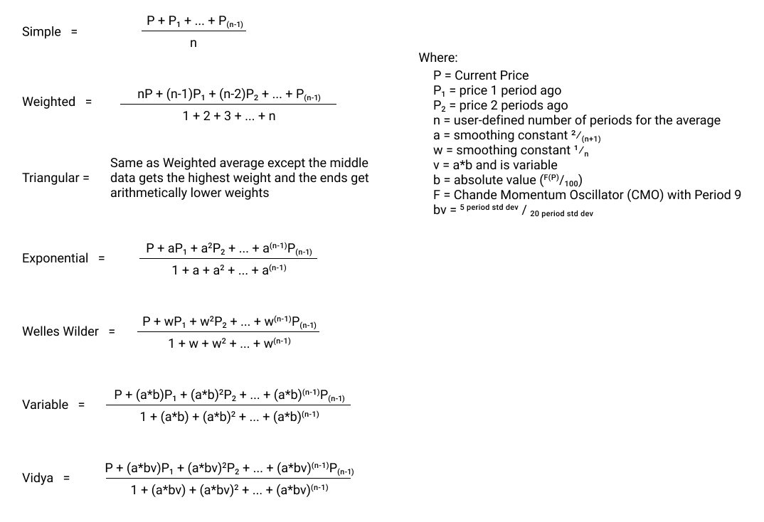
The Moving Average study supports eleven algorithms which increase/decrease the sensitivity of the study, often focusing on more recent data as follows:
-
Simple (SMA): mean (average) of the data.
- R(i)=(X(i)+X(i-1)+X(i-2)+…+X(i-N+1))/N
-
Double Exponential (DEMA)
- R(j)=2*EMA(i,X,N) - EMA(i,EMA(i,X,N),N)
-
Exponential (EMA): newer data are weighted more heavily geometrically.
-
m=2/(N+1)
-
if number of points < N, R(i)=SMA(i,X,number of points)
-
R(i)=m*X(i)+(1-m)*R(i-1)
-
-
Hull (HMA)
-
N’=N/2 rounded up to nearest whole number
-
N’’=sqrt(N) rounded down to nearest whole number
-
MMA(i)=2*WMA(i,X,N’)-WMA(i,X,N)
-
R(i)=WMA(i,MMA,N’’)
-
-
Time Series (TSMA): Calculates a linear regression trendline using the “least squares fit” method.
-
Part of the Linear Regression series, it’s the same as the Forecast
-
SC(i)=X(i)+X(i-1)+X(i-2)+…+X(i-N+1)
-
SWC(i)=N*X(i)-SC(i-1)
-
SW=N*(N+1)/2
-
b(i)=(N*SWC(i)-SW*SC(i))/(N*(SW^3)*(2*N+1)/3)
-
a(i)=(SC(i)-b(i)*SW)/N
-
R(i)=a(i)+b(i)*N
-
-
Triangular (TMA): This is a double SMA. Weighted average where the middle data are given the most weight, decreasing linearly to the end points.
-
N’=N/2 rounded up
-
a(i)=SMA(i,X,N’)
-
If N is even, N’’=N’+1 else N’’=N’
-
R(i)=SMA(i,a,N’’)
-
-
Triple Exponential (TEMA)
- R(j)=3*EMA(i,X,N) - 3*EMA(i,EMA(i,X,N),N) + 3*EMA(i,EMA(i,EMA(i,X,N),N),N)
-
Variable (VMA): An EMA with a volatility index factored into the smoothing formula. The Variable Moving average uses the Chande Momentum Oscillator as the volatility index.
-
Like Welles Wilder, except m= α*β and is variable
-
α=2/(N+1)
-
F=Chande Momentum Oscillator (CMO) with Period 9
-
β=abs(F(i)/100)
-
R(i)=α*β*X(i)+(1-(α*β))*R(i-1)
-
-
VIDYA/Variable Index Dynamic (VDMA): An EMA with a volatility index factored into the smoothing formula. The VIDYA moving average uses the Standard Deviation as the volatility index. (Volatility Index DYnamic Average)
-
Same as VMA except β is different
-
α=2/(N+1)
-
F1(i)=STDEV(i,X,5,SMA) – 5 period Standard Deviation of SMA
-
F2(i)=SMA(i,F1,20) – 20 period SMA of the 5 period STDEV
-
β= F1(i)/F2(i)
-
R(i)=α*β*X(i)+(1-(α*β))*R(i-1)
-
-
Weighted (WMA): newer data are weighted more heavily arithmetically.
-
Most recent data is given most weight, in linear fashion
-
R(i)=N*X(i)+(N-1)*X(i-1)+(N-2)*X(i-2)+…+2*X(i-N+2)+X(i-N+1)
-
-
Welles Wilder (Smoothed, SMMA): The standard EMA formula converts the time period to a fraction using the formula EMA% = 2/(n + 1) where n is the number of days. For example, the EMA% for 14 days is 2/(14 days +1) = 13.3%. Wilder, however, uses an EMA% of 1/14 (1/n) which equals 7.1%. This equates to a 27-day EMA using the standard formula.
-
Same as Exponential except for m:
-
m=1/N
-
R(i)=m*X(i)+(1-m)*R(i-1)
-
- or -
-
R(i)=(X(i)+(N-1)*R(i-1))/N
-
Smoothed Moving Average – Same calculation as an EMA except the smoothing constant is different.
-
P + wP1 + w2P2 + … + w(n-1)P(n-1)
-
1 + w + w2 + … + w(n-1)
-
Exponential smoothing constant: 2/(n+1)
-
Wilder smoothing constant: 1/n
-
Therefore, the Wilder average reacts slower than an exponential average. Also, the Wilder average can be converted into an exponential average with the formula 2n-1. For example, a 26-day Wilder average will draw the exact same plot as a 51-day exponential average.
-
-
Math
Moving Average Convergence/Divergence (MACD)
Indicator Type
Momentum Oscillator
Description
The Moving Average Convergence/Divergence (MACD) indicator makes use of three exponential moving averages (EMA). Two are averages of price and the third is a signal line that is an average of the difference of the other two.
The MACD line is generated from the first two averages, subtracting the longer from the shorter. The Signal Line is simply an EMA of the MACD line. The MACD Histogram measures the spread between the MACD and the Signal line. Changes in direction of the MACD Histogram are often used as early signals of change in trend.
Formula
-
MACD line – short moving average minus long moving average
-
Signal line – a moving average of the MACD line
-
Histogram – measures the difference between the MACD line and the Signal line
Math
- Input Parameters
- Fast MA Period (N2)
- Slow MA Period (N1)
- Signal Period (N3)
- Slow(i) = xMA1(i,X,N1)
- Fast(i) = xMA1(i,X,N2)
- R(i) = Fast(i)-Slow(i)
- Signal(i) = xMA2(i,R,N3)
- Histogram(i) = R(i)-Signal(i)
Moving Average Cross
Indicator Type
- Averages/Bands, Trend Analysis
Description
- Applies three moving averages of the same type to signal changes in trend as the shorter moving averages cross the longer ones.
Math
- See Moving Average
Moving Average Deviation
Indicator Type
Momentum Oscillator
Description
The Moving Average Deviation measures the spread, in points, between the market price and a moving average. The calculation may be shown in either points or percentages.
Related Study: Disparity Index (DI)
Note: This study can be applied to other studies by using the Field parameter.
Math
- Input Parameters
- Period (N)
- Field (X) // Any value displayed on the chart
- Moving average Type (xMA)
- Points or Percent
- MA(i) = xMA(i,X,N)
- R(i) = X(i)-MA(i) if output requested in points
- R(i) = 100*(X(i)/MA(i)-1) if output requested in percentage
Moving Average Envelope
Indicator Type
Moving Average/Bands
Description
The Moving Average Envelope (MAE) plots two lines that form an envelope around a Moving Average of price. The upper and lower bands are a percentage or number of points above and below the moving average.
The MAE can be derived using any of the eleven averaging methodologies supported and may be applied to any data field or study displayed on the chart.
Formula
-
For percentage envelopes:
- Upper band = moving average + x%(moving average)
- Lower band = moving average – x%(moving average)
-
For points envelopes:
- Upper band = moving average + constant
- Lower band = moving average – constant
Math
- Input Parameters
- Period (N)
- Field (X) //Any value displayed on the chart
- Shift Type (Percent or points)
- Shift (S)
- Moving Average Type (xMA)
- Display Settings
- Channel Fill (On/Off)
- %S=percentage shift, pS=point shift
- Rm(i) (median band) = xMA(i,X,N)
- Rt(i) (top band) = Rm(i)+(%S*X(i) + pS) //either %S or pS will be 0
- Rb(i) (bottom band) = Rm(i)-(%S*X(i) + pS)
Negative Volume Index
Indicator Type
Trend Analysis
Description
The Negative Volume Index (NVI) and its sister study, the Positive Volume Index (PVI), are designed to measure the quality of the trend by using volume as a barometer to evaluate the strength of the price action. Price changes on decreasing volume are considered a positive indicator. Whereas, price changes with increasing volume are considered a negative indicator, as increasing trading volumes are more common with retail traders following-the-crowd.
NVI is a moving average of cumulative percentage price changes on periods when volume decreases from bar to bar. For clarity, volume is only used to determine which data points to average, it is not part of the calculation. A trailing moving average of the NVI is used to signal significant changes in trend.
The Negative Volume Index (NVI) was developed by Paul Dysart.
Related Study: Positive Volume Index (PVI)
Note: This study can have other studies applied to it using the Field parameter.
Math
- Input Parameters
- Period (N)
- Field (X) // Any value displayed on the chart
- Moving Average Type (xMA)
- If Volume(i) < Volume(i-1) // negative change in volume
- t(i) = t(i-1)*X(i)/X(i-1)
- otherwise t(i) = t(i-1)
- R(i) = xMA(i,t,N)
On Balance (Cumulative) Volume (OBV)
Indicator Type
Volume, Money Flow
Description
On Balance Volume (OBV) is a cumulative total of the daily volume which sums the volume on days when price rises and subtracts the volume on down days. OBV is often used as a confirmation indicator that shows if the volume activity is supporting the trend.
Related Study: Trade Volume Index (TVI)
Formula
A running total of volume on up-periods minus volume on down periods. Periods with no change have no effect.
OBV = ∑volume * (direction of price change)
Note: Value will change depending on span chosen but plot will look the same.
Math
- D(i):
- if Close(i)-Close(i-1)>0, D(i)=1
- else if Close(i)-Close(i-1)<0, D(i)=-1
- else, D(i)=0
- R(i) = Volume(i)*D(i)+Volume(i-1)*D(i-1) + Volume(i-2)*D(i-2)+…+Volume(0)*D(0)
Option Sentiment by Strike
Indicator Type
Volume, Support/Resistance
Description
The Option Sentiment by Strike study overlays a profile of the volume or open interest of option contracts at each strike price for a security’s most current data point. Calls and puts are graphed as separate, adjacent horizontal bars, allowing the user to understand any bias within the two option types.
Displaying the actual market activity within a security’s corresponding derivative market allows the user to understand positioning and bias within that market. The study may be combined with any other price-based analytics to understand market support and resistance points.
Math
As reported options volume and open interest data for each option strike.
Parabolic SAR
Indicator Type
Trend Analysis, Support/Resistance
Description
The Parabolic SAR indicator is a stop and reverse (SAR) strategy that is designed to highlight when a trend has stalled indefinitely or reversed direction.
The initial SAR is set at the extreme price of the previous trend. After the initial SAR is set, the next interval’s SAR is adjusted in the direction of the trend by the distance between the high for the new trend and the previous SAR then multiplied by an acceleration factor (AF). This is then added to the prior period’s SAR. The acceleration factor typically starts at .02 and increases by .02 to a typical maximum of .20 each period the market makes a new high/low for the move.
When price crosses above the SAR point, the entire calculation starts over but the extreme point becomes the Lowest Low of the new trend and the AF becomes a negative number. The reverse is true when price crosses below.
Formula
For a rising trend:
-
Previous SAR: The SAR value for the previous period.
-
Extreme Point (EP): The Highest High of the current uptrend.
-
Acceleration Factor (AF): Starting at .02
Current SAR = Previous SAR + Previous AF(Previous EP – Previous SAR)
Reversing: Current SAR = Previous SAR – Previous AF(Previous EP – Previous SAR)
Math
- Input Parameters
- Minimum AF (Step)
- Maximum AF (maxStep) //step<maxStep
- LT=true or false, begins at false
- af begins at 0, ep at null
- if LT=false:
- if ep=null or ep>Low(i):
- ep=Low(i-1)
- af=min(af+step,maxStep)
- SAR(i)=SAR(i-1)+af*(ep-SAR(i-1))
- if SAR(i)<High(i):
- SAR(i)=ep
- af=0
- ep=null
- if ep=null or ep>Low(i):
- LT=true
- Else:
- SAR(i)=max(SAR(i),max(High(i-1),High(i-2)))
- Else:
- else if LT=true:
- if ep=null or ep<High(i):
- ep=High(i-1)
- af=min(af+step,maxStep)
- SAR(i)=SAR(i-1)+af*(ep-SAR(i-1))
- if SAR(i)>Low(i):
- SAR(i)=ep
- af=0
- ep=null
- LT=false
- Else:
- SAR(i)=min(SAR(i),min(Low(i-1),Low(i-2)))
- if ep=null or ep<High(i):
- R(i)=SAR(i)
Performance Index (PI)
Indicator Type
Compare; Trend Analysis
Description
The Performance Index (PI) study measures the relative strength of a security to the relative strength of a selected comparison security. Specifically, the PI derives the relative strength, price divided by a moving average, for both the primary series and the comparison series. The PI is the comparison of these two internal relative strength measures. As a ratio, the PI oscillates around 1.00, with positive values indicating strength of the primary security as compared to the benchmark comparison.
Related Study:Price Relative (Relative Strength)
Formula
PRel = Close / SMAClose
CompRel = Comp / SMAComp
PI = (PRel) / (CompRel)
Math
- Input Parameters
- Period (N)
- Comparison symbol (Comp)
- If Comp(i)=0 or no quote then Comp(i)=Comp(i-1)
- R(i) = (Close(i)/Comp(i)) * (SMA(i,Comp(i),N)/SMA(i,Close(i),N))
Pivot Points
Indicator Type
Support/Resistance
Description
Pivots points are used to identify support, resistance and targets, most frequently on intraday charts. The Pivot Points study plots 7 horizontal lines for each period, one for the Pivot line, 3 support levels, and 3 resistance levels. The pivot point itself is simply the average of the high, low and closing prices from the previous trading period. In the subsequent period, trading above the pivot point is thought to indicate ongoing bullish sentiment, while trading below the pivot point indicates bearish sentiment. Pivot points are determined using a longer periodicity than the data displayed on the chart.
Formula
The pivot point and its support and resistance pairs are defined as follows, ordered from highest to lowest:
- H, L, C are the previous period’s High, Low and Close
- Third resistance level (R3) = P + 2*(H – L)
- Second resistance level (R2) = P + (H – L)
- First resistance level (R1) = (2 * P) – L
- Pivot point (P) = (H + L + C) ÷ 3
- First support level (S1) = (2 * P) – H
- Second support level (S2) = P – (H – L)
- Third support level (S3) = P – 2*(H-L)
The period which is used to determine the pivot points is as follows:
- Intraday chart from 1 minute up to but not including 30 minutes – Period=daily
- Intraday chart from 30 minutes upwards – Period=weekly
- Daily charts – Period=monthly
- Weekly and Monthly charts – Period=yearly
Note: Daily periods begin at midnight ET for equities, 5PM for forex, 6PM for metals
Math
- Input Parameters
- Type (Standard or Fibonacci)
- Display Settings
- Continuous (On/Off)
- Shading (On/Off)
- Plots 7 horizontal lines for each period, one for Pivot line, 3 for Support, and 3 for Resistance
- Period is determined as follows:
- Intraday chart from 1 minute up to but not including 30 minutes – Period=daily
- Intraday chart from 30 minutes upwards – Period=weekly
- Daily charts – Period=monthly
- Weekly and Monthly charts – Period=yearly
- Daily periods begin at midnight EST for equities, 5PM for forex, 6PM for metals
- hh=Highest High in the Period
- ll=Lowest Low in the Period
- For each period i:
- Rp(i)=(hh(i)+ll(i)+Close(i))/3
- For Standard Pivot Points:
- Rr1(i)=2*Rp(i)-ll
- Rr2(i)=Rp(i)+hh-ll
- Rr3(i)=Rp(i)+2*(hh-ll)
- Rs1(i)=2*Rp(i)-hh
- Rs2(i)=Rp(i)+ll-hh
- Rs3(i)=Rp(i)+2*(ll-hh)
- For Fibonacci Pivot Points:
- Rr1(i)= Rp(i)+.382*(hh-ll)
- Rr2(i)=Rp(i)+.618*(hh-ll)
- Rr3(i)=Rp(i)+(hh-ll)
- Rs1(i)= Rp(i)+.382*(ll-hh)
- Rs2(i)=Rp(i)+.618(*ll-hh)
- Rs3(i)=Rp(i)+(ll-hh)
Positive Volume Index (PVI)
Indicator Type
Trend Analysis
Description
The Positive Volume Index (PVI) and its sister study, the Negative Volume Index (NVI), are designed to measure the quality of the trend by using volume as a barometer to evaluate the strength of the price action. Price changes on decreasing volume are considered a positive indicator. Whereas, price changes with increasing volume are considered a negative indicator, as increasing trading volumes are more common with retail traders following-the-crowd.
PVI is a moving average of cumulative percentage price changes on periods when volume increases from bar to bar. For clarity, volume is only used to determine which data points to average, it is not part of the calculation. A trailing moving average of the PVI is used to signal significant changes in trend.
The Positive Volume Index (PVI) was developed by Paul Dysart.
Related Study: Negative Volume Index
Note: This study can have other studies applied to it using the Field parameter.
Math
- Input Parameters
- Period (N)
- Field (X) // Any value displayed on the chart
- Moving Average Type (xMA)
- If Volume(i) > Volume(i-1) // positive change in volume
- t(i) = X(i)/X(i-1)*t(i-1)
- otherwise t(i) = t(i-1)
- R(i) = xMA(i,t,N)
Pretty Good Oscillator
Indicator Type
Momentum Oscillator
Description
The Pretty Good Oscillator (PGO) evaluates the strength of the trend in terms of the security’s volatility as measured by an average of the True Range (TR). The PGO calculates the spread of the current close from a simple moving average of the close. This value is normalized by dividing by an exponential moving average of the TR.
The Pretty Good Oscillator was created by Mark Johnson.
Formula
- PGO = (Close - SMA of close) ÷ EMA of True Range
Math
- Input Parameters
- Period (N)
- ma1(i) = EMA(i,TR,N) //TR=True Range
- ma2(i) = SMA(i,Close,N)
- R(i) = (Close(i)-ma2(i))/ma1(i)
Price Momentum Oscillator (PMO)
Indicator Type
Momentum Oscillator
Description
The Price Momentum Oscillator (PMO) is a twice smoothed exponential moving average (EMA) of the percent change of price over one period. The PMO is an unbounded oscillator as it is based on the trend in one period percent changes. An EMA of the PMO is overlaid to provide a signal line to detect significant changes in the PMO oscillator.
Note: This study can be applied to other studies by using the Field parameter.
Formula
- EMA (EMA ( 1 period Percent Change in Price, n ), n2 )
Math
- Input Parameters
- Field (X) //Any value displayed on the chart
- Smoothing Period (N)
- Double Smoothing Period (N2)
- Signal Period (NSig)
- ROC(i) = 1000*(X(i)/X(i-1)-1)
- E(i) = EMA(i,ROC,N-1)
- R(i) = EMA(i,E,N2-1)
- Signal(i) = EMA(i,R,Nsig)
Price Oscillator
Indicator Type
Momentum Oscillator
Description
The Price Oscillator measures the spread between two moving averages, similar to a MACD. Accordingly, it is an unbounded oscillator which measures trend strength. An advantage of the Price Oscillator is it allows the selection of Field, Moving Average Type, and derivation in Points or Percent.
Unlike the MACD, the Price Oscillator does not display a Signal Line or a Histogram.
Related Study: Moving Average Convergence/Divergence (MACD), Rapid Adaptive Variance Indicator (RAVI)
Note: This study can be applied to other studies by using the Field parameter.
Formula
- PO = short moving average minus long moving average
Math
- Input Parameters
- Field (X) //Any value displayed on the chart
- Short Cycle (N1)
- Long Cycle (N2)
- Moving Average Type (xMA)
- Points or Percent
- Short(i) = xMA(i,X,N1)
- Long(i) = xMA(i,X,N2)
- R(i) = Short(i)-Long(i) if output requested in points
- R(i) = 100*(Short(i)/Long(i)-1) if output requested in percentage
Price Rate of Change
Indicator Type
Momentum Oscillator
Description
Price Rate of Change measures the percent change in price over a set range. It is an unbounded oscillator similar to Momentum.
Related Study: Momentum
Note: This study can be applied to other studies by using the Field parameter.
Formula
ROC = Current Price – Price (n-periods ago) -1 * 100 ÷ Price n-periods ago
Math
- Input Parameters
- Period (N)
- Field (X) //Any value displayed on the chart
- R(i) = 100*((X(i)/X(i-N))-1) // optional offset available in code
Price Relative (Relative Strength)
Indicator Type
Comparison, Relative performance
Description
Price Relative is a simple ratio of security A (the loaded security) divided by security B. A rising line indicates security A is out-performing security B and vice-versa.
Formula
- A simple ratio of the first instrument to the second: A / B
Math
- Input Parameters
- Comparison Symbol (Comp)
- If Comp(i)=0 or no quote then Comp(i)=Comp(i-1)
- R(i)=Close(i)/Comp(i)
Price Volume Trend (PVT)
Indicator Type
Money Flow
Description
The Price Volume Trend (PVT) is an aggregation of volume multiplied by price percent change over one period. Significant price moves result in large moves in PVT. The intent of the PVT is to assess the supply/demand balance and volume executed in rising markets versus falling markets.
Formula
PVT = Aggregate( Volume * 1 bar price percent change )
Math
- Input Parameters
- Field (X) // Any value displayed on the chart
- R(i) = R(i-1)+Volume(i)*(X(i)-X(i-1))/X(i-1)
Prime Number Bands (PNB)
Indicator Type
Averages/Bands, Support/Resistance
Description
Prime numbers are often considered magnetic points for price. Accordingly, the Prime Number Bands (PNB) indicator plots the nearest prime number above and below the market price. Spikes in the upper or lower PNB are often considered swing points in the market as it implies the market has failed to break through a prime number.
Math
- If High or Low < 1, then
- pH(i) = # times High(i) needs to be multiplied by 10 to be >10
- pL(i) = # times Low(i) needs to be multiplied by 10 to be >10
- primeH(i) = nearest prime number above High(i)*(10^pH(i))
- primeL(i) = nearest prime number below Low(i)*(10^pL(i))
- Rt(i) = primeH(i)/(10^pH(i))
- Rb(i) = primeL(i)/(10^pL(i))
Prime Number Oscillator
Indicator Type
Statistical, Trend Analysis
Description
Prime numbers are often considered magnetic points for price. Accordingly, the Prime Number Oscillator (PNO) simply identifies if the closest prime number is above (+1) or below (-1) the market on the assumption that the market will gravitate toward that value.
Math
- Input Parameters
- Tolerance Percentage (TP)
- If High or Low < 1, then
- pH(i) = # times High(i) needs to be multiplied by 10 to be >10
- pL(i) = # times Low(i) needs to be multiplied by 10 to be >10
- primeH(i) = nearest prime number above High(i)*(10^pH(i))
- primeL(i) = nearest prime number below Low(i)*(10^pL(i))
- Rt(i) = primeH(i)/(10^pH(i))
- Rb(i) = primeL(i)/(10^pL(i))
- tol(i) = TP*(Rt(i)-Rb(i))/100
- sk(i) = Rt(i)+Rb(i)-2*Close(i)
- Rosc(i) = 1 if sk(i)<tol(i), -1 if sk(i)>tol(i), 0 if sk(i)=tol(i)
Pring’s Know Sure Thing (KST)
Indicator Type
Momentum Oscillator
Description
Created by Martin Pring, The Know Sure Thing (KST) is an unbounded oscillator which sums together four smoothed Rate of Change oscillators with different periodicities into a single measure, the KST line. The use of multiple periodicities results in a very stable oscillator reducing the potential for false signals. The trading signals are generated when the KST line crosses above/below its signal line, a simple moving average of the KST. The KST can also be used to determine overbought and oversold conditions.
KST operates on the principle that price trends are determined by confluence or divergence of many different time cycles and price trend reversals. As a result, the KST formula is weighted in favor of longer time spans.
Note: This study can be applied to other studies by using the Field parameter.
Math
- Input Parameters
- Field (X) //Any value displayed on the chart
- Lightest Rate of Change Period (RP1)
- Light Rate of Change Period (RP2)
- Heavy Rate of Change Period (RP3)
- Heaviest Rate of Change Period (RP4)
- Lightest SMA (N1)
- Light SMA (N2)
- Heavy SMA (N3)
- Heaviest SMA (N4)
- Signal Period (Nsig)
- roc1(i) = 100*(X(i)/X(i-RP1)-1)
- roc2(i) = 100*(X(i)/X(i-RP2)-1)
- roc3(i) = 100*(X(i)/X(i-RP3)-1)
- roc4(i) = 100*(X(i)/X(i-RP4)-1)
- sma1(i) = SMA(i,roc1,N1)
- sma2(i) = SMA(i,roc2,N2)
- sma3(i) = SMA(i,roc3,N3)
- sma4(i) = SMA(i,roc4,N4)
- R(i) = 1*sma1(i)+2*sma2(i)+3*sma3(i)+4*sma4(i)
- Signal(i) = SMA(i,R,Nsig)
Pring’s Special K
Indicator Type
Momentum Oscillator
Description
Created by Martin Pring, the Special K is an unbounded momentum indicator that sums several different weighted averages of twelve rate-of-change calculations. The intent of combining the short-, intermediate- and long-term velocity into one series is to give a view of the true strength of the trend.
Special K serves two functions. First, it identifies reversals in the primary trend relatively early. Second, it uses that information to time short-term pro-trend price moves.
Special K operates on the principle that price trends are determined by confluence or divergence of many different time cycles and price trend reversals. As a result, the formula incorporates rate-of-change calculations using data from years in the past.
Note: This study can be applied to other studies by using the Field parameter.
Math
- Input Parameters
- Field (X) //Any value displayed on the chart
- Interval (Daily/Weekly)
- 12 ROCs, 12 MAs
- Zr = 12 ROC periods:
- For daily series, 10,15,20,30,50,65,75,100,195,265,390,530
- For weekly series, 4,5,6,8,10,13,15,20,39,52,78,104
- Zs = 12 MA periods:
- For daily series, 10,10,10,15,50,65,75,100,130,130,130,195
- For weekly series, 4,5,6,8,10,13,15,20,26,26,26,39
- roc(i) = 100*(X(i)/X(i-Zr)-1) //need to do this 12 times
- ma(i): need to compute 12 ma(i) values, using the 12 roc(i) values and the 12 Zs values of the same index.
- if daily series, SMA(i,roc(i),Zs)
- if weekly series, EMA(i,roc(i),Zs)
- R(i) = 1*ma1(i)+2*ma2(i)+3*ma3(i)+4*ma4(i)
- +1*ma5(i)+2*ma6(i)+3*ma7(i)+4*ma8(i)
- +1*ma9(i)+2*ma10(i)+3*ma11(i)+4*ma12(i)
Projected Aggregate Volume (PAV)
Indicator Type
Volume, Projection
Description
Projected Aggregate Volume (PAV) study is an aggregation of the day’s trading volume up to the current time along with a projection of the aggregate volume for the remainder of the trading day. The PAV study reveals whether the trend in trading volume is above or below average and provides a forecast of volume for the rest of the day.
The anchor time control allows the user to set the starting time of the study to understand how the volume is aggregated from that time forward.
Note: This study is displayed ONLY for intraday periodicities.
Related Study: Projected Volume at Time (PVAT)
Formula
User selects:
- Time Slice (T), the increment of time (< 1 day) over which the study will calculate trading volume
- Lookback Days (L), the number of previous market days to include in the calculation
- Anchor Time (A), the time to start each day (by default, the start of the trading day)
Projected Aggregate Volume (PAV) calculates:
- For each day, D(n), from the start of the lookback period to the current one:
- For each time slice, S(m), in that day from the anchor time (A) to the market close:
- Days = the number of days from D(0) to D(n) that the market was open at S(m)
- Total = the sum of the trading volumes, V(i), of S(m) for each day from D(0) to D(n)
- Avg = Total/Days
- Aggregate Volume (AggVol) = the sum of the volumes of each time slice that day from A to S(m), which PAV displays as a bar chart
- Aggregate Average Volume (AggAvg) = the some of the average volumes of each time slice that day from A to S(m), which PAV displays as a step chart and projects to the end of the current trading day
- For each time slice, S(m), in that day from the anchor time (A) to the market close:
Math
- Input Parameters
- Time Slice (T)
- Lookback Days (L)
- Anchor Time (A)
- For D(n) from D(0) to D(L-1)
- For S(m) from S(A) to S(close)
- Avg(m) = Vol(i) + Vol(i+1) + ... Vol(m)/m
- AggVol(m) = Vol(i) + Vol(i+1) + ... Vol(m)
- AggAvg(m) = Avg(i) + Avg(i+1) + ... Avg(m)
- For S(m) from S(A) to S(close)
Projected Volume at Time (PVAT)
Indicator Type
Volume, Projection
Description
Projected Volume at Time (PVAT) is an average of intraday trading volume for each given time segment. The study highlights whether today’s volume for any particular segment is above or below average. PVAT projects the volume for each time segment for the remainder of the day. A bar graph shows the volume at each periodicity interval (candle); an overlay line shows the average volume for each time segment.
The anchor time control allows the user to set the starting time of the study. If the volume for a given time segment exceeds the threshold multiplier of the average for that time it will be highlighted in yellow (default color).
Note: This study is displayed ONLY for intraday periodicities.
Related Study: Projected Aggregate Volume (PAV)
Formula
User selects:
- Time Slice (T), the increment of time (< 1 day) over which the study will calculate trading volume
- Lookback Days (L), the number of previous market days to include in the calculation
- Anchor Time (A), the time to start each day (by default, the start of the trading day)
- Alert Threshold (H), the minimum percentage difference (positive or negative) between the moving average (MA) and the volume of a particular T that will trigger an alert
- By default, H = +50%
Projected Volume at Time (PVAT) calculates:
- For each day, D(n), from the start of the lookback period to the current one:
- For each time slice, S(m), in that day from the anchor time (A) to the market close:
- Days = the number of days from D(0) to D(n) that the market was open at S(m)
- Total = the sum of the trading volumes, V(i), of S(m) for each day from D(0) to D(n)
- Avg = Total/Days
- If the V(n), the volume of S(m) on D(n) differs from its Avg by more than the alert threshold, H, PVAT displays that volume bar in the alert color
- For each time slice, S(m), in that day from the anchor time (A) to the market close:
Math
- Input Parameters
- Time Slice (T)
- Lookback Days (L)
- Anchor Time (A)
- Alert Threshold (H)
- For D(n) from D(0) to D(L-1)
- For S(m) from S(A) to S(close)
- Avg = V(i) + V(i+1) + ... V(n)/n
- For S(m) from S(A) to S(close)
- If V(n) - Avg > H or Avg - V(n) > |H|, alert
Psychological Line (PL)
Indicator Type
Trend Analysis
Description
The Psychological Line measures the percentage of bars with rising closing prices relative to the prior bar over the defined period. Values above 50% indicate buyers are in control pushing prices higher whereas a value below 50% indicates weakness as sellers are pushing prices lower on average.
Math
- Input Parameters
- Period (N)
- Dup(i) = 1 if Close(i)-Close(i-1)>0, else 0
- R(i) = (100/N)*(Dup(i)+Dup(i-1)+Dup(i-2)+...+Dup(i-N+1))
QStick
Indicator Type
Trend Analysis
Description
The QStick indicator is a moving average of close-open. It measures the average height of the body of a candle, providing insight to the internal strength of the market.
Math
- Input Parameters
- Period (N)
- Moving Average Type (xMA)
- R(i) = xMA(i,Close-Open,N)
Rainbow Moving Average (RMA)
Indicator Type
- Moving Averages/Bands
Description
The Rainbow Moving Average (RMA) study displays ten smoothed simple moving averages (SMA) overlaid on price. The first SMA is calculated on price, each subsequent average smooths the prior SMA using the same range parameter. The averages are color-coded with red being the first average and purple as the smoothest/slowest average.
The RMA can be used to identify trend strength and signal reversals. The trend is strongest when all the SMAs are rising or falling. A reversal is signaled when the faster averages cross all of the slower averages. Consolidation is seen when the averages converge and the spread between them collapses.
Note: This study can be applied to other studies by using the Field parameter.
Formula
RMA10 = SMA (SMA (SMA (SMA (SMA (SMA (SMA (SMA (SMA (SMA (Price,N) ,N) ,N) ,N) ,N) ,N) ,N) ,N) ,N) ,N)
Math
- Input Parameters
- Period (N)
- Field (X) //Any value displayed on the chart
- s1 = SMA(i,X,N)
- s2 = SMA(i,s1,N)
- s3 = SMA(i,s2,N)
- …
- s10 = SMA(i,s9,N)
- s1-s10 are all overlaid on the chart with different colors.
Rainbow Oscillator (RO)
Indicator Type
- Momentum Oscillator
Description
The Rainbow Oscillator (RO) study is a price oscillator that is normalized by the price range. The RO measures the spread of the last price to the average of the ten simple moving averages (SMAs) which is then divided by the range of Highest High-Lowest Low (HH-LL) over the selected period. The result is a momentum oscillator that is normalized by the magnitude of the market’s movement. That is, during a trend both the numerator and the denominator will increase in value, whereas in a consolidation both will decrease.
The RO histogram is displayed within upper and lower bands which mirror one another. Similar to the RO, the Bands measure the spread between the highest and lowest SMA, this value is normalized by the HH-LL range as well.
The Rainbow Oscillator was developed by Mel Widner.
Note: This study can be applied to other studies by using the Field parameter.
Related Study: Rainbow Moving Average (RMA)
Formula
RO Histogram = (Price - Avg of 10 SMAs) / HH-LL Over Lookback
RO Upper = (Max of 10 SMAs - Min of 10 SMAs) / HH-LL Over Lookback
RO Lower = -1 * RO Upper
Math
- Input Parameters
- Period (N)
- Field (X) //Any value displayed on the chart
- HHV/LLV Lookback (L) //lookback period for highest/lowest close
- RMA
- s1 = SMA(i,X,N)
- s2 = SMA(i,s1,N)
- s3 = SMA(i,s2,N)
- …
- s10 = SMA(i,s9,N)
- RMA Oscillator
- acc(i) = s1(i)+s2(i)+s3(i)+…+s10(i)
- mx(i) = max(s1(i),s2(i),s3(i),…,s10(i))
- mn(i) = min(s1(i),s2(i),s3(i),…,s10(i))
- hh = max(Close(i),Close(i-1),Close(i-2),…,Close(i-L+1))
- ll = min(Close(i),Close(i-1),Close(i-2),…,Close(i-L+1))
- R(i) = 100*(X(i)-acc(i)/10)/(hh-ll) //Displayed as a histogram
- Bands are drawn above and below:
- B1(i) = 100*(mx(i)-mn(i))/(hh-ll)
- B2(i) = -B1(i)
Random Walk Index (RWI)
Indicator Type
Statistical, Trend Strength
Description:
The Random Walk Index (RWI) is a statistical indicator that helps determine if the current trend is statistically significant or if it is closer to behaving randomly. RWI plots two lines, a High and a Low, which measure the upward and downward trends, respectively. A significant divergence of the High and Low lines indicates a non-random trend is underway. Spikes in either line indicate a trend corresponding to that line. When the High and Low lines are hovering toward the bottom or close together, it indicates more random behavior. A value of zero in either line indicates the trend in the opposite direction has likely reached an extreme point.
Math
- Input Parameters
- Period (N)
- ttr(0)=0, maxHigh(0)=0, maxLow(0)=0
- for j=1 to N:
- ttr(j) = ttr(j-1)+TR(i-j) //TR=True Range
- denom(j) = (ttr(j)/j)*(j^.5)
- cH(j) = (High(i)-Low(i-j))/denom(j)
- cL(j) = (High(i-j)-Low(i))/denom(j)
- maxHigh(j) = max(maxHigh(j-1),cH(j))
- maxLow(j) = max(maxLow(j-1),cL(j))
- Rh(i) = maxHigh(N)
- Rl(i) = maxLow(N)
Rapid Adaptive Variance Indicator (RAVI)
Indicator Type
Momentum Oscillator
Description
The Rapid Adaptive Variance Indicator (RAVI) measures the percent difference between two moving averages. RAVI is an unbounded oscillator that is similar to the Price Oscillator and MACD, except the result is in percent. In addition it is displayed as a histogram with colored bars which indicate the moving averages are diverging and above/below the Overbought/Oversold level which indicates a trend is in place and accelerating.
Note: This study can be applied to other studies by using the Field parameter.
Related Study: Price Oscillator
Formula
RAVI = short moving average divided by long moving average
Math
- Input Parameters
- Field (X) // Any value displayed on the chart
- Moving Average Type (xMA)
- Short Cycle (N1)
- Long Cycle (N2)
- Display Settings
- Show Zones (Show/Hide)
- OB=Overbought threshold
- OS=Oversold threshold
- Short(i) = xMA(i,X,N1)
- Long(i) = xMA(i,X,N2)
- R(i) = 100*(Short(i)/Long(i)-1)
- if R(i)>OB and R(i-1)<R(i)
- display with INCREASING BAR color
- else if(R(i)<OS and R(i-1)>R(i) display with DECREASING BAR color
- else display with gray color
Relative Strength Index (RSI)
Indicator Type
Momentum Oscillator
Description
The Relative Strength Index (RSI) measures trend strength by using a ratio of average size of the net increases over the past “n” periods and relative to the average size of the net decreases. The result is a bounded oscillator that is indexed between 0 and 100 and is displayed with Overbought and Oversold levels. RSI values are smoothed exponentially using the same “n” period parameter.
The RSI was developed by J. Welles Wilder Jr.
Related Study: Intraday Momentum Index
Note: This study can be applied to other studies by using the Field parameter.
Formula
RS = Average of the up closes over n-periods ÷ Average of the down closes over n-periods
RSI = 100 – 100 ÷ (1 + RS)
Math
- Input Parameters
- Period (N)
- Field (X)
- Display Settings
- Show Zones (On/Off)
- OverBought
- OverSold
- d(i) = X(i)-X(i-1)
- p(i): max(0,d(i))
- n(i): min(0,d(i))
- avgP(i) = (avgP(i-1)*(N-1)+p(i))/N
- avgL(i) = (avgL(i-1)*(N-1)-n(i))/N
- R(i) = 100-(100/(1+(avgP(i)/avgL(i)))) // or - 100*(avgP(i)/(avgP(i)+avgL(i)))
- * if avgL(i)=0 then R(i)=100
Relative Strength
Indicator Type
Compare; Trend Analysis
Description
The Relative Strength study measures the percent change between the leftmost and rightmost bars of a series or study relative to another symbol or comparison series. It displays the magnitude and direction of performance difference using a percent change formula, allowing both positive and negative values. Mountain shading highlights gains (positive regions) and losses (negative regions) with customizable colors for enhanced visual analysis.
Formula
RS = [(Right Close - Left Close) / Left Close] × 100
Relative Vigor Index (RVI)
Indicator Type
Momentum Oscillator
Description
The Relative Vigor Index (RVI) study compares a Triangular Moving Average (TMA) of the close-open (candle bodies) to a TMA of the high-low range. The RVI rises when the close is near the highs and the open is near the lows. Candle bodies are close in size to the high-low range of the period. The converse is true in down trends.
A TMA of the RVI is used as a signal line to indicate significant change in trend. In addition, a histogram is displayed which measures the spread between the RVI and its Signal line.
Formula
RVI = Sum (TriangularMA of Body,N) ÷ Sum (TriangularMA of HL Range,N)
Signal = TMA (RVI,4)
RVI Hist = RVI - Signal
Math
- Input Parameters
- Period (N)
- ma1(i) = TMA(i,Close-Open,4) //Average Body
- ma2(i) = TMA(i,High-Low,4) //Average HL Range
- s1(i) = ma1(i)+ma1(i-1)+ma1(i-2)+…+ma1(i-N+1)
- s2(i) = ma2(i)+ma2(i-1)+ma2(i-2)+…+ma2(i-N+1)
- if s2 = 0 then s2=.00000001
- R(i) = s1(i)/s2(i)
- Signal(i) = TMA(i,R,4)
- RV_Hist(i) = R(i)-Signal(i) //Green bars when increasing spread, red when decreasing
Relative Volatility
Indicator Type
Volatility
Description
Relative Volatility measures the standard deviation of price changes over a set lookback range. The value is then normalized into a percentage, with overbought and oversold lines being marked at 70% and 30%, respectively. Readings above 50 indicate upward volatility, while readings below 50 indicate downward volatility.
It is similar to the Relative Strength Index (RSI), which looks at the close instead of the standard deviation.
Note: This study can be applied to other studies by using the Field parameter.
Math
- Input Parameters
- Field (X) //Any value displayed on the chart
- STD Period (S)
- Smoothing Period (N)
- s(i) = STDEV(i,X,S,SMA) //5 period Standard Deviation of SMA
- avgP:
- if X(i)>X(i-1) then avgP(i)=(avgP(i-1)*(N-1)+s(i))/N
- else avgP(i)= avgP(i-1)*(N-1)/N
- avgL:
- if X(i)>X(i-1) then avgL(i)=avgL(i-1)*(N-1)/N
- else avgL(i)=(avgL(i-1)*(N-1)+s(i))/N
- R(i) = 100*avgP(i)/(avgP(i)+avgL(i))
- if avgP(i)+avgL(i)=0 then R(i)=100
Schaff Trend Cycle (STC)
Indicator Type
Momentum Oscillator
Description
The Schaff Trend Cycle (STC) is designed to be a forward-looking, leading indicator that generates faster, more reactive and accurate signals than other indicators. The STC is a double smoothed stochastic of the MACD creating a bounded oscillator between 0 - 100.
The STC will remain in Overbought or Oversold territory for long stretches of time producing limited information when a market is trending. Crossing above 25 or below 75 are the key signals generated by the STC.
The Schaff Trend Cycle was developed by Doug Schaff.
Note: This study can be applied to other studies by using the Field parameter.
Math
- Input Parameters
- Period (N)
- Field (X) //Any value displayed on the chart
- Short Cycle
- Long Cycle
- Moving Average Type (xMA)
- N1,N2 - Periods
- Short(i) = xMA(i,X,N1)
- Long(i) = xMA(i,X,N2)
- macd(i) = Short(i)-Long(i)
- H(i) = Highest macd value over last N periods including current bar
- L(i) = Lowest macd value over last N periods including current bar
- f1 and f2 start at 0
- f1(i): if H(i)>L(i) then 100*(macd(i)-L(i))/(H(i)-L(i)) else
f1(i-1) - PF starts at f1
- PF(i): if PF(i-1)!=0 then PF(i-1)+.5*(f1(i)-PF(i-1)) else f1
- H’(i) = Highest PF value over last N periods including current bar
- L’(i) = Lowest PF value over last N periods including current bar
- f2(i): if H’(i)>L’(i) then 100*(PF(i)-L’(i))/(H’(i)-L’(i)) else
f2(i-1) - R(i): if R(i-1) then R(i-1)+.5*(f2(i)-R(i-1)) else f2
Shinohara Intensity Ratio (SIR)
Indicator Type
Trend Analysis
Description
The Shinohara Intensity Ratio (SIR) displays Strong (Strength) and Weak Ratio (Popularity) lines which are similar to the +DI and -DI of the ADX/DMS study. Market strength is indicated when the SIR Strong Ratio is above the SIR Weak Ratio.
The Weak Ratio is a moving sum of the High-Close divided by Close-Low. In a bull market when the Close is typically above the midpoint of the bar the numerator High(i)-Close(i) will be less than the denominator Close(i)-Low(i) resulting in smaller values that are summed.
The Strong Ratio is a moving sum of a bar’s High less the prior bar’s Close divided by the prior Close less the Low. This captures the true directional strength of a trend as prices should advance/decline from one period to the next. Accordingly, the Strong Ratio will follow the market. A change in direction of the Strong Ratio suggests that a trend may be reversing and a cross of the Weak Ratio indicates an emerging trend.
Formula
Weak Ratio = Sum ( (High-Close) / (Close-Low), N)
Strong Ratio = Sum ( (High-Close(-1)) / (Close(-1)-Low), N)
Math
- Input Parameters
- Period (N)
- Weak(i) = (High(i)-Close(i))/(Close(i)-Low(i))
- Strong(i) = (High(i)-Close(i-1))/(Close(i-1)-Low(i))
- Rw(i) = 100*(Weak(i)+Weak(i-1)+Weak(i-2)+…+Weak(i-N+1))
- Rs(i) = 100*(Strong(i)+Strong(i-1)+Strong(i-2)+…+ Strong(i-N+1))
Standard Deviation
Indicator Type
Statistical
Description
The Standard Deviation indicator is a statistical measure of variability, it is frequently used to assess market volatility. A low standard deviation indicates that the data points tend to be very close to the mean which occurs when the market is consolidating. A high standard deviation value indicates significant dispersion of the data points which often occurs when trends are ending.
Note: This study can be applied to other studies by using the Field parameter.
Math
- Input Parameters
- Period (N)
- Field (X)
- Standard Deviations (M)
- Moving Average Type (xMA)
- ma(i) = xMA(i,X,N)
- acc1(i) = (X(i)^2)+(X(i-1)^2)+(X(i-2)^2)+…+(X(i-N+1)^2)
- acc2(i) = X(i)+X(i-1)+X(i-2)+…+X(i-N+1)
- R(i) = (((acc1(i)+N*(ma(i)^2)-2*ma(i)*acc2(i))/N)^.5)*M
STARC Bands
Indicator Type
Moving Averages/Bands, Volatility
Description
The STARC (Stoller Average Range Channel) Bands are similar to ATR Bands, except the bands are centered on a simple moving average (SMA) instead of the last close. STARC plots the SMA with upper and lower bands based on recent volatility as measured by Average True Range (ATR). The Bands are calculated using a set percentage multiple (±S) of the ATR which is added/subtracted to the SMA.
When the price breaks out of the channel, it can be interpreted as a signal. Given the center line is a moving average instead of last price, the bands are far more stable than the ATR Bands.
Related Study: Average True Range (ATR), ATR Trailing Stop, True Range (TR), ATR Bands
STARC Bands were developed by Manning Stoller.
Formula
M is the ATR period, N is the SMA period
Median Band = SMA(i, Close, N)
Top band = Median Band + %Shift * ATR(M)
Bottom Band = Median Band - %Shift * ATR(M)
Math
- Input Parameters
- Period (AM) //ATR Period
- MA Period (N)
- Multiplier (%S) //percentage shift
- Rm(i) = SMA(i,Close,N) //median band
- Rt(i) = Rm(i)+(%S*ATR(i)) //top band
- Rb(i) = Rm(i)-(%S*ATR(i)) //bottom band
Stochastics
Indicator Type
Momentum Oscillator
Description
The Stochastics indicator is a bounded oscillator that normalizes price within a range by measuring the percentage distance of the last price relative to the upper and lower bounds of its recent trading range. That is, the Stochastic equals 0 when price is at the bottom of the range and 100 when it is at the top. The Fast version (%K) of the Stochastic simply measures where price is in its range. The Slow version (%D) of Stochastic applies a simple moving average (SMA) (typically, 3 period) to remove the volatility of the oscillator and reduce the number of signals generated.
The %D is a trailing trigger line which is a SMA of the %K Stochastic line. The Stochastic values range from 0 to 100. The Overbought and Oversold levels default to 80 and 20 respectively.
The Stochastic Oscillator was developed by George C. Lane.
Related Study: Williams %R, Stochastic Momentum (SMI)
Note: This study can be applied to other studies by using the Field parameter.
Formula
Calculates where price is within a recent range.
-
Fast calculation (%K) uses raw value with a SMA
-
Slow (smoothed) version (%D) uses the simple average with another simple average of the first
Fast %K = (Current Price – Lowest Low) / (Highest High – Lowest Low)
Fast %D = SMA( Fast %K)
Slow %K = Fast %D
Slow %D = SMA( Slow %K )
Math
- Input Parameters
- Field (X) //Any value displayed on the chart
- %K Periods (NK)
- Fast (On/Off)
- If Fast = Off: %K Smoothing Periods (NKS)
- %D Periods (ND)
- Display Settings
- Show Zones (On/Off)
- Overbought //default = 80
- Oversold //default = 20
- hh = HHV(i+1,NK) //Highest High over NK periods including current bar
- ll = LLV(i+1,NK) //Lowest Low over NK periods including current bar
- If Fast is selected:
- st(i) = 100*(X(i)-ll)/(hh-ll)
- Else, st(i) = SMA(i,st,NKS) //smoothing of %K
- Rf(i) = st(i)
- Rs(i) = SMA(i,st,ND) //trigger line
Stochastic Momentum (SMI)
Indicator Type
Momentum Oscillator
Description
The Stochastic Momentum (SMI) is a variation on the original Stochastic indicator, both of which are bounded oscillators designed to identify Overbought and Oversold conditions. The SMI measures price relative to the median of its recent range, rather than a percentage location within the range as done for the Stochastic. The SMI is positive when price is above the median and negative when below it. In addition the SMI uses EMAs to smooth and stabilize the output.
The %D is a moving average of the %K SMI line which provides trigger line that helps to confirm the directional signals. The SMI oscillator values range from -100 to 100 with Overbought and Oversold thresholds defaulted to 40 and -40, respectively.
The SMI was developed by William Blau.
Math
- Input Parameters
- %K Periods (NK)
- %K Smoothing Period (NK1)
- %K Double Smoothing Period (NK2)
- %D Periods (ND)
- %D Moving Average Type (xMA)
- Display Settings
- Show Zones (On/Off)
- Overbought //default = 80
- Oversold //default = 20
- hh=HHV(i+1,NK) //Highest High over NK periods including current bar
- ll=LLV(i+1,NK) //Lowest Low over NK periods including current bar
- H(i) = Close(i)-(hh-ll)/2
- DHL(i) = hh-ll
- maHS1(i) = EMA(i,H,NK1)
- maHS2(i) = EMA(i,maHS1,NK2)
- maDHL1(i) = EMA(i,DHL,NK1)
- maDHL2(i) = EMA(i,maDHL1,NK2)
- RpK(i) = 100*maHS2(i)/(.5*maDHL2(i)) //This is %K
- RpD(i) = xMA(i,RpK,ND) //This is %D
Supertrend
Indicator Type
Trend Analysis, Support/Resistance
Description
The Supertrend indicator is a trailing stop tool which plots either a support line below the market or a resistance line above the market, based on the market trend. The Supertrend will switch lines when the high or low price intersects with the plotted line, similar to the Parabolic SAR indicator.
The upper line is the median price plus a multiple of Average True Range (ATR). Similarly, the lower line is the median price minus a multiple of the ATR. Similar to any trailing stop, the upper line follows the market lower and will never move higher once established. Conversely, the lower line follows the market higher and will never move lower once established.
Arrows are drawn pointing to the close of the bar when the direction changes and the bands flip.
Formula
Upper = ((high + low ÷ 2) + Multiplier * ATR) …Only if price < upper
Lower = ((high + low ÷ 2) – Multiplier * ATR) …Only if price > lower
Math
- Input Parameters
- Period (N)
- Multiplier (M)
- uptrend(i) = median price(i)-ATR(i)*M
- if(Close(i-1)>uptrend(i-1)>uptrend(i)) then uptrend(i)=uptrend(i-1)
- downtrend(i) = median price(i)+ATR(i)*M
- if(Close(i-1)<downtrend(i-1)<downtrend(i)) then downtrend(i)=downtrend(i-1)
- direction(i) = direction(i-1)
- if(Close(i)>downtrend(i-1)) then direction(i) changes to 1
- if(Close(i)<uptrend(i-1)) then direction(i) changes to -1
- R(i) = uptrend(i) if direction(i)=1, or downtrend(i) if direction(i)=-1
- R(i) is plotted in two colors:
- Red (or other Downtrend color) when direction(i)=-1
- Green (or other Uptrend color) when direction(i)=1
- Arrows are drawn pointing to the Close of the bar on the ticks where direction changes
Swing Index (SI)
Indicator Type
Trend Analysis, Momentum Oscillator
Description
The Swing Index indicator (SI) uses last two bars data to identify market swings that may signal a change in trend over a longer period of time. Accordingly, each period’s value is independent from prior values. The SI compares the action from the current high/low to the prior close as well as the current range and open-close body of the current and prior bars. The short term nature of the SI make is useful as an early warning signal highlighting that investors are changing their trading behavior setting up for a potential change in trend.
The Swing Index was developed by Welles Wilder.
Related Study: Accumulative Swing Index (ASI)
Math
- Input Parameters
- T = Limit Move Value; if not supplied, 99999
- A(i) = abs(High(i)-Close(i-1)) //Strength
- B(i) = abs(Low(i)-Close(i-1)) //Weakness
- C(i) = abs(High(i)-Low(i)) //Range
- D(i) = abs(Close(i-1)-Open(i-1)) //prior range of body
- K(i) = max(A(i),B(i)) //Prior close to extreme HL
- M(i) = max(C(i),K(i)) //Range or Prior close to extreme HL
- r(i) = M(i)+D(i)/4 //Swing+Prior Body
- if M = A
- then r(i) = r(i)-B(i)/2
- else if M = B
- then r(i) = r(i)-A(i)/2
- S(i) = (50*( (Close(i)-Close(i-1))+(Close(i)-Open(i))/2 + (Close(i-1)-Open(i-1))/4) ÷ r(i))*K(i) ÷ T
- Swing Index: R(i) = S(i)
Time Series Forecast
Indicator Type
Statistical, Moving Averages/Bands
Description
The Linear Regression Forecast (LRF) uses the ordinary least squares method to derive a linear function which plots a straight line through prices so as to minimize the distances between the prices and the resulting trendline. The last point of the trendline is the forecasted value. The LRF is a moving series which plots the forecasted value of the derived trend line each period, thereby following the market like a moving average.
Related Study: Linear Regression Forecast
Note: This study can be applied to other studies by using the Field parameter.
Math
- Input Parameters
- Period (N)
- Field (F)
- SC(i) = X(i)+X(i-1)+X(i-2)+…+X(i-N+1)
- SWC(i) = N*X(i)-SC(i-1)
- SW = N*(N+1)/2
- b(i) = (N*SWC(i)-SW*SC(i))/(N*(SW^3)*(2*N+1)/3)
- a(i) = (SC(i)-b(i)*SW)/N
- Rf(i) = a(i)+b(i)*N //Forecast
Trade Volume Index (TVI)
Indicator Type
Money Flow
Description
Trade Volume Index (TVI) adds a price movement threshold parameter to the On Balance Volume (OBV) study. Accordingly, like OBV, TVI is a cumulative total of the volume with the difference being that it only sums the volume on periods when price rises to a minimum threshold and subtracts the volume on down periods that exceed the threshold. TVI is often used as a confirmation indicator that shows if the volume activity is supporting the trend.
Related Study: On Balance (Cumulative) Volume (OBV)
Formula
A running total of volume on up-periods minus volume on down periods of when the absolute value of price change meets a minimum threshold. Periods with no change have no effect.
TVI = ∑volume * (direction of price change) …incomplete
Note: Value will change depending on span chosen but plot will look the same.
Math
- Input Parameters
- Minimum Tick Value (MT) // in points
- D(i):
- if Close(i)-Close(i-1)>MT, D(i)=1
- else if Close(i)-Close(i-1)<MT, D(i)=-1
- else, D(i)=D(i-1)
- R(i) = Volume(i)*D(i)+Volume(i-1)*D(i-1) + Volume(i-2)*D(i-2)+…+Volume(0)*D(0)
Trend Intensity Index (TII)
Indicator Type
Momentum Oscillator
Description
The Trend Intensity Index (TII) is a ratio of the sum of price deviation above a simple moving average relative to the sum of the price deviation below a simple moving average. The TII is a bounded oscillator between 0 and 100. The TII will move to an extreme value during strong trends.
Formula
TII = total up ÷ (total up + total down) × 100
TII Signal = EMA ( TII, n-period )
Math
- Input Parameters
- Period (N)
- Field (X) // Any value displayed on the chart
- Signal Period (K)
- d(i) = X(i)-SMA(i,X,N)
- p(i): max(0,d(i))
- n(i): min(0,d(i))
- gain(i) = p(i)+p(i-1)+p(i-2)+…+p(i-N/2) // (N/2 is rounded up)
- loss(i) = n(i)+n(i-1)+n(i-2)+…+n(i-N/2) // (N/2 is rounded up)
- R(i) = 100-(100/(1+(gain(i)/loss(i)))) // - or - 100*(gain(i)/(gain(i)+loss(i)))
- * if loss(i)=0 then R(i)=100
- Signal(i) = EMA(i,R,K)
TRIX Oscillator
Indicator Type
Momentum Oscillator
Description
The TRIX Oscillator measures the percent change of the triple exponential moving average (TEMA) of the close from one bar to the next. A central benefit of the TRIX oscillator when compared to others is it is quite smooth, providing greater clarity of the signals.
The TRIX Oscillator was developed by Jack Hutson.
Formula
- EMA3 = EMA(EMA(EMA(Close)))
- TRIX = 100 * ( EMA3(i) ÷ EMA3(i-1) - 1 )
Math
- Input Parameters
- Period (N)
- E3(i) = EMA(i,EMA(i,EMA(i,Close,N),N),N)
- R(i) = 100*(E3(i) ÷ E3(i-1)-1)
True Range (TR)
Indicator Type
Volatility
Description
The derivation of the True Range (TR) captures gap openings that are missed by traditional high-low ranges.
Related Study: ATR Bands, Average True Range (ATR)
Formula
The TR is defined as the greatest of:
- Current High – Previous Close
- Previous Close – Current Low (absolute value)
- Current High – Current Low (absolute value)
Math
- R(i) = max(High(i),Close(i-1))-min(Low(i),Close(i-1))
Twiggs Money Flow (TMF)
Indicator Type
Volume, Money Flow
Description
Developed by Colin Twiggs, the Twiggs Money Flow (TMF) indicator is a moving sum of volume, displayed as an oscillator, weighted by where price closes within its range. The indicator oscillates around 0, with positive amounts indicating a bullish trend, and negative amounts indicating a bearish trend.
The TMF is a derivation of the Chaikin Money Flow (CMF) indicator, which is in turn derived from the Accumulation/Distribution line. There are two primary differences between TMF and CMF. The first is that the TMF volume multiplier is derived using the True Range instead of the H-L range. The second is TMF is derived using moving averages instead of cumulative volume. Consequently, these two indicators produce similar results.
Math
- Input Parameters
- Period (N)
- TRh(i) = max(High(i),Close(i-1))
- TRl(i) = min(Low(i),Close(i-1))
- MFV(i) = Volume(i)*(2*Close(i)-TRh(i)-TRl(i)) / (TRh(i)-TRl(i))
- if TRh(i)-TR(l)=0 then divide by 999999 instead
- sMFV(i) = MFV(i)+(MFV(i-1)+MFV(i-2)+…+MFV(i-N+1))/N
- sVol(i) = Volume(i)+(Volume(i-1)+Volume(i-2)+…+Volume(i-N+1))/N //SMA of volume
- R(i) = sMFV(i)/sVol(i)
- if sVol(i) = 0 then divide by 999999 instead
Extra Materials
For more information, please go to: http://www.incrediblecharts.com/indicators/twiggs_money_flow.php
Typical Price (TP)
Indicator Type
Moving Averages/Bands
Description
The Typical Price indicator is a simple moving average (SMA) of the mean of the high, low, and close.
Note: The term “Typical Price” is used throughout technical analysis in other studies where it refers to HLC3, whereas the Typical Price Indicator is an SMA of HLC3.
Formula
TP = SMA (( high + low + close ) ÷ 3,n-bars )
Math
- Input Parameters
- Period (N)
- t(i) = (High(i)+Low(i)+Close(i))/3
- R(i) = (t(i)+t(i-1)+t(i-2)+…+t(i-N+1))/N
Ulcer Index
Indicator Type
- Volatility, Trend Analysis
Description
The Ulcer Index measures the depth of a drawdown from a recent high. Specifically, as stated by Peter Martin: it is the square root of the mean of the squared percentage drawdowns in value. The squaring effect penalizes large drawdowns proportionately more than small drawdowns.
The Ulcer Index was developed by Peter Martin and Byron McCann.
Note: This study can be applied to other studies by using the Field parameter.
Math
- Input Parameters
- Period (N)
- Field (X) //Any value displayed on the chart
- h(i) = max(X(i),X(i-1),X(i-2),…,X(i-N+1))
- PD2(i) = (100*(X(i)/h(i)-1))^2 // Square of “% Drawdown”
- R(i) = SMA(i,PD2,N)^.5
Ultimate Oscillator
Indicator Type
- Momentum Oscillator
Description
The Ultimate Oscillator (UO) indicator is designed to improve the Overbought and Oversold signals by capturing the market’s momentum across three different time periods (i.e., Cycles). The UO effectively averages oscillators across three periodicities. The UO is a bounded oscillator with values between 0 and 100. Divergences between the UO and market price are often considered an important signal that the trend is failing and will reverse.
The Ultimate Oscillator was developed by Larry Williams.
Math
- Input Parameters
- Cycle 1 (C1)
- Cycle 2 (C2)
- Cycle 3 (C3)
- C12 = C1*C2
- C23 = C2*C3
- C13 = C1*C3
- minLC(i) = min(Low(i),Close(i-1))
- bp(i) = Close(i)-minLC(i)
- tr(i) = max(High(i),Close(i-1))-minLC(i)
- accbp(i,x) = bp(i)+bp(i-1)+bp(i-2)+…+bp(i-Cx+1) //x represents 1,2, or 3. The formula is applied once for each value of x.
- acctr(i,x) = tr(i)+tr(i-1)+tr(i-2)+…+tr(i-Cx+1)
- num(i) = C23*accbp(i,1)/acctr(i,1)+C13*accbp(i,2)/acctr(i,2)+C12*accbp(i,3)/acctr(i,3)
- R(i) = num(i)/C23*C13*C12
Valuation Lines
Indicator Type
- Averages/Bands, Statistical
Description
The Valuation Line is an average of all the data points displayed on the chart. Accordingly, the value will change as the data on the chart is panned left/right or expanded or compressed. Any Field shown on the chart may be selected as the input, including other studies. Three average types are supported: Mean, Median, Harmonic.
Standard Deviation bands may also be displayed above/below the average.
Note: This study can be applied to other studies by using the Field parameter.
Math
- Input Parameters
- Field (X)
- Average Type (xMA)
- Display Settings
- 1 Standard Deviation
- 2 Standard Deviations
- 3 Standard Deviations
- R(i) = (X(i)+X(i-1)+X(i-2)+…+X(i-n+1)) ÷ n //n is defined by the number of data points shown not a user input
Vertical Horizontal Filter (VHF)
Indicator Type
- Trend Analysis
Description
The Vertical Horizontal Filter (VHF) is a measure of trend extension and consolidation. It is a ratio of high-low over a range of time divided by the sum of the absolute value of price changes. Higher values indicate a stronger trend, lower values indicate a consolidation.
The Vertical Horizontal Filter was created by Adam White.
Formula
Parameter: n periods
VHF = (Highest High(n) - Lowest Low(n)) ÷ Sum of 1 period net change
for n periods
Math
- Input Parameters
- Period (N)
- hh = HHV(i+1,N) // Highest High starting at current bar
- ll = LLV(i+1,N) // Lowest Low starting at current bar
- ch(i) = ABS(Close(i)-Close(i-1))
- R(i) = (hh-ll)/(ch(i)+ch(i-1)+ch(i-2)+…+ch(i-N+1))
Volatility Cone
Indicator Type
Volatility, Projection
Description
The Volatility Cone indicator displays a cone projected forward with the likely price range based on recent volatility. Either historical or implied volatility (if available) may be used as the input. The Volatility Projection Cone is a forward-looking study that allows users to blend information from the options market with other technical analysis tools.
Math
- Input Parameters
- Volatility source // historical or implied
- Probability 68% (1σ) // checkbox
- Probability 95% (2σ) // checkbox
- Projection Bars // how far cone projects
- Days per year (Dt) // how many days to use for annualization
- P - current price
V - annualized volatility (historical or implied)n
n - Projection bar
- UpperValue1σ = P + V * sqrt(n / Dt)
- LowerValue1σ = P - V * sqrt(n / Dt)
Volume Chart
Indicator Type
Volume
Description
Volume is used to quantify trading activity each period in a market, market sector, or individual instrument. It can be added as an underlay on the chart or in a separate window.
Related Study: Volume Underlay
Formula
As reported data.
Volume Oscillator (VO)
Indicator Type
Volume
Description
The Volume Oscillator (VO) measures the spread between two exponential moving averages of volume, which is similar to a Price Oscillator using volume as the field.
Formula
VO = EMA ( Volume, short period ) minus EMA ( Volume long period )
Math
- Input Parameters
- Short Cycle (N1)
- Long Cycle (N2)
- Points or Percent
- Short(i) = xMA(i,Vol,N1)
- Long(i) = xMA(i,Vol,N2)
- R(i) = Short(i)-Long(i) // if output requested in points
- R(i) = 100*(Short(i)/Long(i)-1) // if output requested in percentage
Volume Profile
Indicator Type
Volume, Support/Resistance
Description
Volume Profile, sometimes called “volume at price”, overlays horizontal volume bars extending from the y-axis. It is designed to show the volume traded at each price level over the span of the chart. Volume Profile is often used to identify possible support and resistance.
The High-Low range for the date:time range displayed is divided by the number of buckets resulting in a high and low of each bucket. For each time period, the volume value is examined and that volume is placed into the bucket whose high value < volume value and low value > volume value.
The Volume Profile only considers the range of data shown on the screen and will change if the chart is stretched, squeezed, or scrolled back or forward in time. By combining volume and price, the user can identify high-volume price ranges which indicate price levels where significant volume was transacted indicating a balanced market. These levels are likely to provide support or resistance in the future.
Math
- Input Parameters
- Price Buckets (N)
- Display Settings
- Width Percentile
- Display Border
- Display Volume
As reported data.
Volume Rate of Change
Indicator Type
Volume
Description
Volume Rate of Change measures the percent change in volume over a set range.
Related Study: Price Rate of Change
Formula
VROC = Current Volume – Volume (n-periods ago) * 100 -1 ÷ Volume n-periods ago
Math
- Input Parameters
- Period (N)
- R(i) = 100*((X(i)/X(i-N))-1)
Volume Underlay
Indicator Type
Volume
Description
Volume is used to quantify trading activity each period in a market, market sector, or individual instrument. It can be added as an underlay on the chart or in a separate window.
Related Study: Volume Chart
Formula
As reported data.
Volume Weighted Average Price (VWAP)
Indicator Type
Volume, Moving Averages/Bands
Description
The Volume-Weighted Average Price (VWAP) is an intraday moving average that is weighted by the volume. It is used to get a view of the fair value of the market based on the price at which volume was executed on average throughout a single day’s trading session. The calculation starts when trading opens and ends when it closes.
The VWAP multiplies the volume for each period times the typical price (HLC3). Because it also divides by the total volume, the VWAP is considered distinct from the simple moving average (SMA).
VWAP is often used as a confirmation tool in combination with other indicators, and has many uses. For example, a stock trading at prices below the VWAP may be seen as undervalued.
Related Study: Anchored VWAP
Math
- HLC3(i) = (High(i)+Low(i)+Close(i)/3)
- Vcum(i) = SUM (Volume(i)) //for the day
- PVcum(i) = SUM (HLC3(i)*Volume(i)) //for the day
- R(i) = PVcum(i)/Vcum(i)
Vortex Indicator (VI)
Indicator Type
Trend Analysis
Description
The Vortex Indicator (VI) evaluates the strength of the trend by measuring the upside and downside price action. Accordingly, the VI derives an Uptrend line (+VI) and a Downtrend line (-VI). Positive price movement is measured over two bars by subtracting the prior low from the current high. The +VI is the sum of the upside values divided by the sum of the True Range (TR) for each bar.
Conversely, negative price movement subtracts the prior high from the current low. The -VI is the sum of the downside values divided by the sum of the TR for each bar.
The crossover of the +VI and -VI is often considered the signal of a new trend in the direction of the rising VI line.
The Vortex Indicator was created by Etienne Botes and Douglas Siepman.
Formula
+VI = Sum ( High - Prior Low, n-bars) ÷ Sum ( True Range, n-bars )
-VI = Sum ( Low - Prior High, n-bars) ÷ Sum ( True Range, n-bars )
Math
- Input Parameters
- Period (N)
- pVM(i) = High(i)-Low(i-1)) // H - prior L
- nVM(i) = Low(i)-High(i-1)) // Low - prior H
- spVM(i) = pVM(i)+pVM(i-1)+pVM(i-2)+…+pVM(i-N)
- snVM(i) = nVM(i)+nVM(i-1)+nVM(i-2)+…+nVM(i-N)
- sTR(i) = TR(i)+TR(i-1)+TR(i-2)+…+TR(i-N) // True Range
- Rp(i) = spVM(i)/sTR(i) // positive VI
- Rn(i) = snVM(i)/sTR(i) // negative VI
Weighted Close (WC)
Indicator Type
Moving Average/Bands
Description
The Weighted Close indicator is a simple moving average of the period’s high, low, and close, with close receiving double weight given its importance of mark-to-market.
Formula
WC = SMA( ( high + low + close*2 ) ÷ 4, N-bars )
Math
- Input Parameters
- Period (N)
- t(i) = (High(i)+Low(i)+2*Close(i))/4
- R(i) = (t(i)+t(i-1)+t(i-2)+…+t(i-N+1))/N
Williams %R
Indicator Type
Momentum Oscillator
Description
The Williams %R indicator normalizes prices within a range by measuring the percentage distance of the last price relative to the upper and lower bounds of its recent trading range. The result is multiplied by -100 and is plotted on a scale of -100 to zero.
The Williams %R indicator was developed by Larry Williams.
Related Study: Stochastics
Formula
%R = (Highest High – Current) / (Highest High – Lowest Low) * -100
Math
- Input Parameters
- Period (N)
- hh = HHV(i+1,N) //Highest High starting at current bar
- ll = LLV(i+1,N) //Lowest Low starting at current bar
- R(i) = 100*(hh-Close(i))/(hh-ll)
ZigZag
Indicator Type
Trend Analysis
Description
The ZigZag study identifies price swings of a predefined minimum magnitude. It is designed to filter out noisy fluctuations in price while identifying larger trends in which the market advances or declines by a minimum percentage (D). ZigZag is effective for analyzing historical data, and cannot forecast future trends.
The trend lines are drawn when price movement exceeds a distance threshold percentage. A Lowest Low point is recorded once the upward price movement achieves the percentage distance threshold from the low. Conversely, a Highest High point is recorded once the downward price is reached which achieves the minimum percentage magnitude.
For OHLC data, the high and low values of the bar are considered. For line and mountain charts, only the close is considered.
The final leg of the ZigZag is a proposed line between the last extreme value encountered and the present price.
Formula
- Input Parameter
- D = Distance %
- R(i)=collection of Highest Highs and Lowest Lows which are distance>=D from each other.
For example, a Lowest Low is recorded once a high is reached which is D greater than that low, after which Lowest Low is sought once more. A Highest High is recorded once a low is reached which is D less than that high, after which Highest High is sought once more. - The final leg runs from the last extreme in R(i) to the present price.
- Lowest low/Highest High become lowest close/highest close when viewing a chart which only displays the close